Geodesics in Kerr spacetime¶

Geodesics of Kerr spacetime are implemented via the class KerrGeodesic.

class kerrgeodesic_gw.kerr_geodesic.KerrGeodesic(parent, initial_point, pt0=None, pr0=None, pth0=None, pph0=None, mu=None, E=None, L=None, Q=None, r_increase=True, th_increase=True, chart=None, name=None, latex_name=None, a_num=None, m_num=None, verbose=False)¶

Bases: sage.manifolds.differentiable.integrated_curve.IntegratedGeodesic

Geodesic of Kerr spacetime.

Geodesics are computed by solving the geodesic equation via the generic SageMath geodesic integrator.

INPUT:

parent – IntegratedGeodesicSet, the set of curves \(\mathrm{Hom_{geodesic}}(I, M)\) to which the geodesic belongs
initial_point – point of Kerr spacetime from which the geodesic is to be integrated
pt0 – (default: None) Boyer-Lindquist component \(p^t\) of the initial 4-momentum vector
pr0 – (default: None) Boyer-Lindquist component \(p^r\) of the initial 4-momentum vector
pth0 – (default: None) Boyer-Lindquist component \(p^\theta\) of the initial 4-momentum vector
pph0 – (default: None) Boyer-Lindquist component \(p^\phi\) of the initial 4-momentum vector
mu – (default: None) mass \(\mu\) of the particle
E – (default: None) conserved energy \(E\) of the particle
L – (default: None) conserved angular momemtum \(L\) of the particle
Q – (default: None) Carter constant \(Q\) of the particle
r_increase – (default: True) boolean; if True, the initial value of \(p^r=\mathrm{d}r/\mathrm{d}\lambda\) determined from the integral of motions is positive or zero, otherwise, \(p^r\) is negative
th_increase – (default: True) boolean; if True, the initial value of \(p^\theta=\mathrm{d}\theta/\mathrm{d}\lambda\) determined from the integral of motions is positive or zero, otherwise, \(p^\theta\) is negative
chart – (default: None) chart on the spacetime manifold in terms of which the geodesic equations are expressed; if None the default chart (Boyer-Lindquist coordinates) is assumed
name – (default: None) string; symbol given to the geodesic
latex_name – (default: None) string; LaTeX symbol to denote the geodesic; if none is provided, name will be used
a_num – (default: None) numerical value of the Kerr spin parameter \(a\) (required for a numerical integration)
m_num – (default: None) numerical value of the Kerr mass parameter \(m\) (required for a numerical integration)
verbose – (default: False) boolean; determines whether some information is printed during the construction of the geodesic

EXAMPLES:

We construct first the Kerr spacetime:

sage: from kerrgeodesic_gw import KerrBH
sage: a = var('a')
sage: M = KerrBH(a); M
Kerr spacetime M
sage: BLchart = M.boyer_lindquist_coordinates(); BLchart
Chart (M, (t, r, th, ph))

We pick an initial spacetime point for the geodesic:

sage: init_point = M((0, 6, pi/2, 0), name='P')

A geodesic is constructed by providing the range of the affine parameter, the initial point and either (i) the Boyer-Lindquist components \((p^t_0, p^r_0, p^\theta_0, p^\phi_0)\) of the initial 4-momentum vector \(p_0 = \left. \frac{\mathrm{d}x}{\mathrm{d}\lambda}\right| _{\lambda=0}\), (ii) the four integral of motions \((\mu, E, L, Q)\) or (iii) some of the components of \(p_0\) along with with some integrals of motion. We shall also specify some numerical value for the Kerr spin parameter \(a\). Examples of (i) and (iii) are provided below. Here, we choose \(\lambda\in[0, 300m]\), the option (ii) and \(a=0.998 m\), where \(m\) in the black hole mass:

sage: geod = M.geodesic([0, 300], init_point, mu=1, E=0.883,
....:                   L=1.982, Q=0.467, a_num=0.998)
sage: geod
Geodesic of the Kerr spacetime M

The numerical integration of the geodesic equation is performed via integrate(), by providing the step in \(\delta\lambda\) in units of \(m\):

sage: geod.integrate(step=0.005)

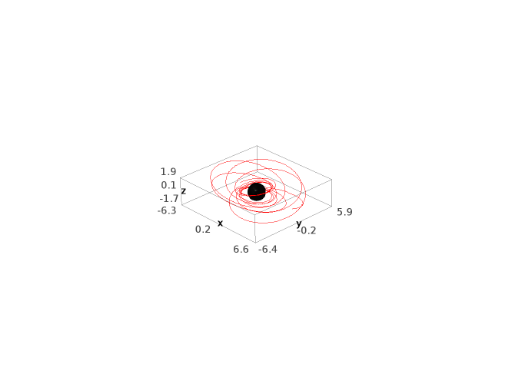
We can then plot the geodesic:

sage: geod.plot()
Graphics3d Object

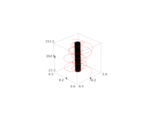
Actually, many options can be passed to plot(). For instance to a get a 3D spacetime diagram:

sage: geod.plot(coordinates='txy')
Graphics3d Object

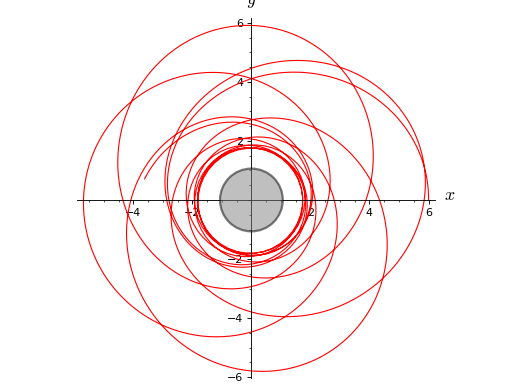
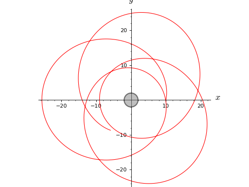
or to get the trace of the geodesic in the \((x,y)\) plane:

sage: geod.plot(coordinates='xy', plot_points=2000)
Graphics object consisting of 2 graphics primitives

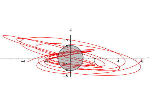
or else to get the trace in the \((x,z)\) plane:

sage: geod.plot(coordinates='xz')
Graphics object consisting of 2 graphics primitives

As a curve, the geodesic is a map from an interval of \(\mathbb{R}\) to the spacetime \(M\):

sage: geod.display()
(0, 300) → M
sage: geod.domain()
Real interval (0, 300)
sage: geod.codomain()
Kerr spacetime M

It maps values of \(\lambda\) to spacetime points:

sage: geod(0)
Point on the Kerr spacetime M
sage: geod(0).coordinates()  # coordinates in the default chart  # tol 1.0e-13
(0.0, 6.0, 1.5707963267948966, 0.0)
sage: BLchart(geod(0))       # equivalent to above   # tol 1.0e-13
(0.0, 6.0, 1.5707963267948966, 0.0)
sage: geod(300).coordinates()   # tol 1.0e-13
(553.4637326813786, 3.703552505462962, 1.6613834863942039, 84.62814710987239)

The initial 4-momentum vector \(p_0\) is returned by the method initial_tangent_vector():

sage: p0 = geod.initial_tangent_vector(); p0
Tangent vector p at Point P on the Kerr spacetime M
sage: p0 in M.tangent_space(init_point)
True
sage: p0.display()  # tol 1.0e-13
p = 1.29225788954106 ∂/∂t + 0.00438084990626460 ∂/∂r
 + 0.0189826106258554 ∂/∂th + 0.0646134478134985 ∂/∂ph
sage: p0[:]  # tol 1.0e-13
[1.29225788954106, 0.00438084990626460, 0.0189826106258554, 0.0646134478134985]

For instance, the components \(p^t_0\) and \(p^\phi_0\) are recovered by:

sage: p0[0], p0[3]  # tol 1.0e-13
(1.29225788954106, 0.0646134478134985)

Let us check that the scalar square of \(p_0\) is \(-1\), i.e. is consistent with the mass parameter \(\mu = 1\) used in the construction of the geodesic:

sage: g = M.metric()
sage: g.at(init_point)(p0, p0).subs(a=0.998)  # tol 1.0e-13
-1.00000000000000

The 4-momentum vector \(p\) at any value of the affine parameter \(\lambda\), e.g. \(\lambda=200m\), is obtained by:

sage: p = geod.evaluate_tangent_vector(200); p
Tangent vector at Point on the Kerr spacetime M
sage: p in M.tangent_space(geod(200))
True
sage: p.display()  # tol 1.0e-13
1.316592599498746 ∂/∂t - 0.07370434215844164 ∂/∂r
 - 0.01091195426423706 ∂/∂th + 0.07600209768075264 ∂/∂ph

The particle mass \(\mu\) computed at a given value of \(\lambda\) is returned by the method evaluate_mu():

sage: geod.evaluate_mu(0)  # tol 1.0e-13
1.00000000000000

Of course, it should be conserved along the geodesic; actually it is, up to the numerical accuracy:

sage: geod.evaluate_mu(300)  # tol 1.0e-13
1.0000117978600134

Similarly, the conserved energy \(E\), conserved angular momentum \(L\) and Carter constant \(Q\) are computed at any value of \(\lambda\) by respectively evaluate_E(), evaluate_L() and evaluate_Q():

sage: geod.evaluate_E(0)  # tol 1.0e-13
0.883000000000000
sage: geod.evaluate_L(0)  # tol 1.0e-13
1.98200000000000
sage: geod.evaluate_Q(0)  # tol 1.0e-13
0.467000000000000

Let us check that the values of \(\mu\), \(E\), \(L\) and \(Q\) evaluated at \(\lambda=300 m\) are equal to those at \(\lambda=0\) up to the numerical accuracy of the integration scheme:

sage: geod.check_integrals_of_motion(300)  # tol 1.0e-13
  quantity         value            initial value       diff.      relative diff.
  $\mu^2$    1.0000235958592163   1.00000000000000    0.00002360     0.00002360
    $E$      0.883067996080701    0.883000000000000   0.00006800     0.00007701
    $L$       1.98248080818931    1.98200000000000    0.0004808      0.0002426
    $Q$      0.467214137649741    0.467000000000000   0.0002141      0.0004585

Decreasing the integration step leads to smaller errors:

sage: geod.integrate(step=0.001)
sage: geod.check_integrals_of_motion(300)  # tol 1.0e-13
  quantity         value            initial value       diff.      relative diff.
  $\mu^2$    1.0000047183936422   1.00000000000000     4.718e-6       4.718e-6
    $E$      0.883013604456676    0.883000000000000   0.00001360     0.00001541
    $L$      1.98209626120918     1.98200000000000    0.00009626     0.00004857
    $Q$      0.467042771975860    0.467000000000000   0.00004277     0.00009159

Various ways to initialize a geodesic

Instead of providing the integral of motions, as for geod above, one can initialize a geodesic by providing the Boyer-Lindquist components \((p^t_0, p^r_0, p^\theta_0, p^\phi_0)\) of the initial 4-momentum vector \(p_0\). For instance:

sage: p0
Tangent vector p at Point P on the Kerr spacetime M
sage: p0[:]  # tol 1.0e-13
[1.29225788954106, 0.00438084990626460, 0.0189826106258554, 0.0646134478134985]
sage: geod2 = M.geodesic([0, 300], init_point, pt0=p0[0], pr0=p0[1],
....:                    pth0=p0[2], pph0=p0[3], a_num=0.998)
sage: geod2.initial_tangent_vector() == p0
True

As a check, we recover the same values of \((\mu, E, L, Q)\) as those that were used to initialize geod:

sage: geod2.evaluate_mu(0)
1.00000000000000
sage: geod2.evaluate_E(0)
0.883000000000000
sage: geod2.evaluate_L(0)
1.98200000000000
sage: geod2.evaluate_Q(0)
0.467000000000000

We may also initialize a geodesic by providing the mass \(\mu\) and the three spatial components \((p^r_0, p^\theta_0, p^\phi_0)\) of the initial 4-momentum vector:

sage: geod3 = M.geodesic([0, 300], init_point, mu=1, pr0=p0[1],
....:                    pth0=p0[2], pph0=p0[3], a_num=0.998)

The component \(p^t_0\) is then automatically computed:

sage: geod3.initial_tangent_vector()[:]  # tol 1.0e-13
[1.29225788954106, 0.00438084990626460, 0.0189826106258554, 0.0646134478134985]

and we check the identity with the initial vector of geod, up to numerical errors:

sage: (geod3.initial_tangent_vector() - p0)[:]  # tol 1.0e-13
[2.22044604925031e-16, 0, 0, 0]

Another way to initialize a geodesic is to provide the conserved energy \(E\), the conserved angular momentum \(L\) and the two components \((p^r_0, p^\theta_0)\) of the initial 4-momentum vector:

sage: geod4 = M.geodesic([0, 300], init_point, E=0.8830, L=1.982,
....:                     pr0=p0[1], pth0=p0[2], a_num=0.998)
sage: geod4.initial_tangent_vector()[:]
[1.29225788954106, 0.00438084990626460, 0.0189826106258554, 0.0646134478134985]

Again, we get a geodesic equivalent to geod:

sage: (geod4.initial_tangent_vector() - p0)[:]  # tol 1.0e-13
[0, 0, 0, 0]

check_integrals_of_motion(affine_parameter, solution_key=None)¶

Check the constancy of the four integrals of motion

INPUT:

affine_parameter – value of the affine parameter \(\lambda\)
solution_key – (default: None) string denoting the numerical solution to use for evaluating the various integrals of motion; if None, the latest solution computed by integrate() is used.

OUTPUT:

a SageMath table with the absolute and relative differences with respect to the initial values.

evaluate_E(affine_parameter, solution_key=None)¶

Compute the conserved energy \(E\) at a given value of the affine parameter \(\lambda\).

INPUT:

affine_parameter – value of the affine parameter \(\lambda\)
solution_key – (default: None) string denoting the numerical solution to use for the evaluation; if None, the latest solution computed by integrate() is used.

OUTPUT:

value of \(E\)

evaluate_L(affine_parameter, solution_key=None)¶

Compute the conserved angular momentum about the rotation axis \(L\) at a given value of the affine parameter \(\lambda\).

INPUT:

affine_parameter – value of the affine parameter \(\lambda\)
solution_key – (default: None) string denoting the numerical solution to use for the evaluation; if None, the latest solution computed by integrate() is used.

OUTPUT:

value of \(L\)

evaluate_Q(affine_parameter, solution_key=None)¶

Compute the Carter constant \(Q\) at a given value of the affine parameter \(\lambda\).

INPUT:

affine_parameter – value of the affine parameter \(\lambda\)
solution_key – (default: None) string denoting the numerical solution to use for the evaluation; if None, the latest solution computed by integrate() is used.

OUTPUT:

value of \(Q\)

evaluate_mu(affine_parameter, solution_key=None)¶

Compute the mass parameter \(\mu\) at a given value of the affine parameter \(\lambda\).

INPUT:

affine_parameter – value of the affine parameter \(\lambda\)
solution_key – (default: None) string denoting the numerical solution to use for the evaluation; if None, the latest solution computed by integrate() is used.

OUTPUT:

value of \(\mu\)

evaluate_mu2(affine_parameter, solution_key=None)¶

Compute the square of the mass parameter \(\mu^2\) at a given value of the affine parameter \(\lambda\).

INPUT:

affine_parameter – value of the affine parameter \(\lambda\)
solution_key – (default: None) string denoting the numerical solution to use for the evaluation; if None, the latest solution computed by integrate() is used.

OUTPUT:

value of \(\mu^2\)

evaluate_tangent_vector(affine_parameter, solution_key=None)¶

Return the tangent vector (4-momentum) at a given value of the affine parameter.

INPUT:

affine_parameter – value of the affine parameter \(\lambda\)
solution_key – (default: None) string denoting the numerical solution to use for the evaluation; if None, the latest solution computed by integrate() is used.

OUTPUT:

instance of TangentVector representing the 4-momentum vector \(p\) at \(\lambda\)

initial_tangent_vector()¶

Return the initial 4-momentum vector.

OUTPUT:

instance of TangentVector representing the initial 4-momentum \(p_0\)

EXAMPLES:

Initial 4-momentum vector of a null geodesic in Schwarzschild spacetime:

sage: from kerrgeodesic_gw import KerrBH
sage: M = KerrBH(0)
sage: BLchart = M.boyer_lindquist_coordinates()
sage: init_point = M((0, 6, pi/2, 0), name='P')
sage: geod = M.geodesic([0, 100], init_point, mu=0, E=1,
....:                   L=3, Q=0)
sage: p0 = geod.initial_tangent_vector(); p0
Tangent vector p at Point P on the Schwarzschild spacetime M
sage: p0.display()
p = 3/2 ∂/∂t + 1/6*sqrt(30) ∂/∂r + 1/12 ∂/∂ph

integrate(step=None, method='odeint', solution_key=None, parameters_values=None, verbose=False, **control_param)¶

Solve numerically the geodesic equation.

INPUT:

step – (default: None) step \(\delta\lambda\) for the integration, where \(\lambda\) is the affine parameter along the geodesic; default value is a hundredth of the range of \(\lambda\) declared when constructing the geodesic
method – (default: 'odeint') numerical scheme to use for the integration; available algorithms are:
- 'odeint' - makes use of scipy.integrate.odeint via Sage solver desolve_odeint(); odeint invokes the LSODA algorithm of the ODEPACK suite, which automatically selects between implicit Adams method (for non-stiff problems) and a method based on backward differentiation formulas (BDF) (for stiff problems).
- 'rk4_maxima' - 4th order classical Runge-Kutta, which makes use of Maxima’s dynamics package via Sage solver desolve_system_rk4() (quite slow)
- 'dopri5' - Dormand-Prince Runge-Kutta of order (4)5 provided by scipy.integrate.ode
- 'dop853' - Dormand-Prince Runge-Kutta of order 8(5,3) provided by scipy.integrate.ode
and those provided by GSL via Sage class ode_solver:
- 'rk2' - embedded Runge-Kutta (2,3)
- 'rk4' - 4th order classical Runge-Kutta
- 'rkf45' - Runge-Kutta-Felhberg (4,5)
- 'rkck' - embedded Runge-Kutta-Cash-Karp (4,5)
- 'rk8pd' - Runge-Kutta Prince-Dormand (8,9)
- 'rk2imp' - implicit 2nd order Runge-Kutta at Gaussian points
- 'rk4imp' - implicit 4th order Runge-Kutta at Gaussian points
- 'gear1' - \(M=1\) implicit Gear
- 'gear2' - \(M=2\) implicit Gear
- 'bsimp' - implicit Bulirsch-Stoer (requires Jacobian)
solution_key – (default: None) string to tag the numerical solution; if None, the string method is used.
parameters_values – (default: None) list of numerical values of the parameters present in the system defining the geodesic, to be substituted in the equations before integration
verbose – (default: False) prints information about the computation in progress
**control_param – extra control parameters to be passed to the chosen solver

EXAMPLES:

Bound timelike geodesic in Schwarzschild spacetime:

sage: from kerrgeodesic_gw import KerrBH
sage: M = KerrBH(0)
sage: BLchart = M.boyer_lindquist_coordinates()
sage: init_point = M((0, 10, pi/2, 0), name='P')
sage: lmax = 1500.
sage: geod = M.geodesic([0, lmax], init_point, mu=1, E=0.973,
....:                   L=4.2, Q=0)
sage: geod.integrate()
sage: geod.plot(coordinates='xy')
Graphics object consisting of 2 graphics primitives

With the default integration step, the accuracy is not very good:

sage: geod.check_integrals_of_motion(lmax)  # tol 1.0e-13
  quantity           value             initial value       diff.     relative diff.
  $\mu^2$      1.000761704316941     1.00000000000000    0.0007617     0.0007617
    $E$       0.9645485805304451     0.973000000000000   -0.008451     -0.008686
    $L$       3.8897905637080923     4.20000000000000     -0.3102       -0.07386
    $Q$      5.673017835722329e-32           0           5.673e-32         -

Let us improve it by specifying a smaller integration step:

sage: geod.integrate(step=0.1)
sage: geod.check_integrals_of_motion(lmax)  # tol 1.0e-13
  quantity           value             initial value        diff.      relative diff.
  $\mu^2$     1.0000101879128696     1.00000000000000    0.00001019      0.00001019
    $E$       0.9729448260004574     0.973000000000000   -0.00005517    -0.00005671
    $L$        4.197973829219027     4.20000000000000     -0.002026      -0.0004824
    $Q$      6.607560764960032e-32           0            6.608e-32          -

We may set the parameter solution_key to keep track of various numerical solutions:

sage: geod.integrate(step=0.1, solution_key='step_0.1')
sage: geod.integrate(step=0.02, solution_key='step_0.02')

and use it in the various evaluation functions:

sage: geod.evaluate_mu(lmax, solution_key='step_0.1')  # tol 1.0e-13
1.0000050939434606
sage: geod.evaluate_mu(lmax, solution_key='step_0.02')  # tol 1.0e-13
1.0000010212056811

plot(coordinates='xyz', prange=None, solution_key=None, style='-', thickness=1, plot_points=1000, color='red', include_end_point=(True, True), end_point_offset=(0.001, 0.001), verbose=False, label_axes=None, plot_horizon=True, horizon_color='black', fill_BH_region=True, BH_region_color='grey', display_tangent=False, color_tangent='blue', plot_points_tangent=10, width_tangent=1, scale=1, aspect_ratio='automatic', **kwds)¶

Plot the geodesic in terms of the coordinates \((t,x,y,z)\) deduced from the Boyer-Lindquist coordinates \((t,r,\theta,\phi)\) via the standard polar to Cartesian transformations.

INPUT:

coordinates – (default: 'xyz') string indicating which of the coordinates \((t,x,y,z)\) to use for the plot
prange – (default: None) range of the affine parameter \(\lambda\) for the plot; if None, the entire range declared during the construction of the geodesic is considered
solution_key – (default: None) string denoting the numerical solution to use for the plot; if None, the latest solution computed by integrate() is used.
verbose – (default: False) determines whether information is printed about the plotting in progress
plot_horizon – (default: True) determines whether the black hole event horizon is drawn
horizon_color – (default: 'black') color of the event horizon
fill_BH_region – (default: True) determines whether the black hole region is colored (for 2D plots only)
BH_region_color – (default: 'grey') color of the event horizon
display_tangent – (default: False) determines whether some tangent vectors should also be plotted
color_tangent – (default: blue) color of the tangent vectors when these are plotted
plot_points_tangent – (default: 10) number of tangent vectors to display when these are plotted
width_tangent – (default: 1) sets the width of the arrows representing the tangent vectors
scale – (default: 1) scale applied to the tangent vectors before displaying them

Geodesics in Kerr spacetime¶

Previous topic

Next topic

This Page