Kerr spacetime

The Kerr black hole is implemented via the class KerrBH, which provides the Lorentzian manifold functionalities associated with the Kerr metric, as well as functionalities regarding circular orbits (e.g. computation of the ISCO, Roche limit, etc.).

REFERENCES:

• J. M. Bardeen, W. H. Press and S. A. Teukolsky, Astrophys. J. 178, 347 (1972), doi:10.1086/151796

• L. Dai and R. Blandford, Mon. Not. Roy. Astron. Soc. 434, 2948 (2013), doi:10.1093/mnras/stt1209

class kerrgeodesic_gw.kerr_spacetime.KerrBH(a, m=1, manifold_name='M', manifold_latex_name=None, metric_name='g', metric_latex_name=None)

Bases: sage.manifolds.differentiable.pseudo_riemannian.PseudoRiemannianManifold

Kerr black hole spacetime.

The Kerr spacetime is generated as a 4-dimensional Lorentzian manifold, endowed with the Boyer-Lindquist coordinates (default chart). Accordingly the class KerrBH inherits from the generic SageMath class PseudoRiemannianManifold.

INPUT:

• a – reduced angular momentum

• m – (default: 1) total mass

• manifold_name – (default: 'M') string; name (symbol) given to the spacetime manifold

• manifold_latex_name – (default: None) string; LaTeX symbol to denote the spacetime manifold; if none is provided, it is set to manifold_name

• metric_name – (default: 'g') string; name (symbol) given to the metric tensor

• metric_latex_name – (default: None) string; LaTeX symbol to denote the metric tensor; if none is provided, it is set to metric_name

EXAMPLES:

Creating a Kerr spacetime with symbolic parameters \((a, m)\):

sage: from kerrgeodesic_gw import KerrBH
sage: a, m = var('a m')
sage: BH = KerrBH(a, m); BH
Kerr spacetime M
sage: dim(BH)
4

The Boyer-Lindquist chart:

sage: BH.boyer_lindquist_coordinates()
Chart (M, (t, r, th, ph))
sage: latex(_)
\left(M,(t, r, {\theta}, {\phi})\right)

The Kerr metric:

sage: g = BH.metric(); g
Lorentzian metric g on the Kerr spacetime M
sage: g.display()
g = -(a^2*cos(th)^2 - 2*m*r + r^2)/(a^2*cos(th)^2 + r^2) dt⊗dt
 - 2*a*m*r*sin(th)^2/(a^2*cos(th)^2 + r^2) dt⊗dph
 + (a^2*cos(th)^2 + r^2)/(a^2 - 2*m*r + r^2) dr⊗dr
 + (a^2*cos(th)^2 + r^2) dth⊗dth
 - 2*a*m*r*sin(th)^2/(a^2*cos(th)^2 + r^2) dph⊗dt
 + (2*a^2*m*r*sin(th)^4 + (a^2*r^2 + r^4 + (a^4 + a^2*r^2)*cos(th)^2)*sin(th)^2)/(a^2*cos(th)^2 + r^2) dph⊗dph
sage: g[0,3]
-2*a*m*r*sin(th)^2/(a^2*cos(th)^2 + r^2)

A Kerr spacetime with specific numerical values for \((a,m)\), namely \(m=1\) and \(a=0.9\):

sage: BH = KerrBH(0.9); BH
Kerr spacetime M
sage: g = BH.metric()
sage: g.display()  # tol 1.0e-13
g = -(r^2 + 0.81*cos(th)^2 - 2*r)/(r^2 + 0.81*cos(th)^2) dt⊗dt
 - 1.8*r*sin(th)^2/(r^2 + 0.81*cos(th)^2) dt⊗dph
 + (1.0*r^2 + 0.81*cos(th)^2)/(1.0*r^2 - 2.0*r + 0.81) dr⊗dr
 + (r^2 + 0.81*cos(th)^2) dth⊗dth
 - 1.8*r*sin(th)^2/(r^2 + 0.81*cos(th)^2) dph⊗dt
 + (1.62*r*sin(th)^4 + (1.0*r^4 + (0.81*r^2 + 0.6561)*cos(th)^2
    + 0.81*r^2)*sin(th)^2)/(1.0*r^2 + 0.81*cos(th)^2) dph⊗dph
sage: g[0,3]
-1.8*r*sin(th)^2/(r^2 + 0.81*cos(th)^2)

The Schwarrzschild spacetime as the special case \(a=0\) of Kerr spacetime:

sage: BH = KerrBH(0, m)
sage: g = BH.metric()
sage: g.display()
g = (2*m - r)/r dt⊗dt - r/(2*m - r) dr⊗dr + r^2 dth⊗dth + r^2*sin(th)^2 dph⊗dph

The object returned by metric() belongs to the SageMath class PseudoRiemannianMetric, for which many methods are available, like christoffel_symbols_display() to get the Christoffel symbols with respect to the Boyer-Lindquist coordinates (by default, only nonzero and non-redundant symbols are displayed):

sage: g.christoffel_symbols_display()
Gam^t_t,r = -m/(2*m*r - r^2)
Gam^r_t,t = -(2*m^2 - m*r)/r^3
Gam^r_r,r = m/(2*m*r - r^2)
Gam^r_th,th = 2*m - r
Gam^r_ph,ph = (2*m - r)*sin(th)^2
Gam^th_r,th = 1/r
Gam^th_ph,ph = -cos(th)*sin(th)
Gam^ph_r,ph = 1/r
Gam^ph_th,ph = cos(th)/sin(th)

or ricci() to compute the Ricci tensor (identically zero here since we are dealing with a solution of Einstein equation in vacuum):

sage: g.ricci()
Field of symmetric bilinear forms Ric(g) on the Schwarzschild
 spacetime M
sage: g.ricci().display()
Ric(g) = 0

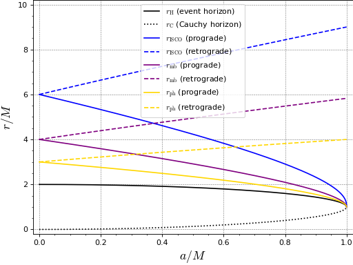
Various methods of KerrBH class implement the computations of remarkable radii in the Kerr spacetime. Let us use them to reproduce Fig. 1 of the seminal article by Bardeen, Press and Teukolsky, ApJ 178, 347 (1972), doi:10.1086/151796, which displays these radii as functions of the black hole spin paramater \(a\). The radii of event horizon and inner (Cauchy) horizon are obtained by the methods event_horizon_radius() and cauchy_horizon_radius() respectively:

sage: graph = plot(lambda a: KerrBH(a).event_horizon_radius(),
....:              (0., 1.), color='black', thickness=1.5,
....:              legend_label=r"$r_{\rm H}$ (event horizon)",
....:              axes_labels=[r"$a/M$", r"$r/M$"],
....:              gridlines=True, frame=True, axes=False)
sage: graph += plot(lambda a: KerrBH(a).cauchy_horizon_radius(),
....:               (0., 1.), color='black', linestyle=':', thickness=1.5,
....:               legend_label=r"$r_{\rm C}$ (Cauchy horizon)")

The ISCO radius is computed by the method isco_radius():

sage: graph += plot(lambda a: KerrBH(a).isco_radius(),
....:               (0., 1.), thickness=1.5,
....:               legend_label=r"$r_{\rm ISCO}$ (prograde)")
sage: graph += plot(lambda a: KerrBH(a).isco_radius(retrograde=True),
....:               (0., 1.), linestyle='--', thickness=1.5,
....:               legend_label=r"$r_{\rm ISCO}$ (retrograde)")

The radius of the marginally bound circular orbit is computed by the method marginally_bound_orbit_radius():

sage: graph += plot(lambda a: KerrBH(a).marginally_bound_orbit_radius(),
....:               (0., 1.), color='purple', linestyle='-', thickness=1.5,
....:               legend_label=r"$r_{\rm mb}$ (prograde)")
sage: graph += plot(lambda a: KerrBH(a).marginally_bound_orbit_radius(retrograde=True),
....:               (0., 1.), color='purple', linestyle='--', thickness=1.5,
....:               legend_label=r"$r_{\rm mb}$ (retrograde)")

The radius of the photon circular orbit is computed by the method photon_orbit_radius():

sage: graph += plot(lambda a: KerrBH(a).photon_orbit_radius(),
....:               (0., 1.), color='gold', linestyle='-', thickness=1.5,
....:               legend_label=r"$r_{\rm ph}$ (prograde)")
sage: graph += plot(lambda a: KerrBH(a).photon_orbit_radius(retrograde=True),
....:               (0., 1.), color='gold', linestyle='--', thickness=1.5,
....:               legend_label=r"$r_{\rm ph}$ (retrograde)")

The final plot:

sage: graph
Graphics object consisting of 8 graphics primitives

Arbitrary precision computations are possible:

sage: a = RealField(200)(0.95) # 0.95 with 200 bits of precision
sage: KerrBH(a).isco_radius()  # tol 1e-50
1.9372378781396625744170794927972658947432427390836799716847

angular_momentum()

Return the reduced angular momentum of the black hole.

EXAMPLES:

sage: from kerrgeodesic_gw import KerrBH
sage: a, m = var('a m')
sage: BH = KerrBH(a, m)
sage: BH.spin()
a

An alias is angular_momentum():

sage: BH.angular_momentum()
a

boyer_lindquist_coordinates(symbols=None, names=None)

Return the chart of Boyer-Lindquist coordinates.

INPUT:

• symbols – (default: None) string defining the coordinate text symbols and LaTeX symbols, with the same conventions as the argument coordinates in RealDiffChart; this is used only if the Boyer-Lindquist chart has not been already defined; if None the symbols are generated as \((t,r,\theta,\phi)\).

• names – (default: None) unused argument, except if symbols is not provided; it must be a tuple containing the coordinate symbols (this is guaranteed if the shortcut operator <,> is used)

OUTPUT:

• the chart of Boyer-Lindquist coordinates, as an instance of RealDiffChart

EXAMPLES:

sage: from kerrgeodesic_gw import KerrBH
sage: a, m = var('a m')
sage: BH = KerrBH(a, m)
sage: BH.boyer_lindquist_coordinates()
Chart (M, (t, r, th, ph))
sage: latex(BH.boyer_lindquist_coordinates())
\left(M,(t, r, {\theta}, {\phi})\right)

The coordinate variables are returned by the square bracket operator:

sage: BH.boyer_lindquist_coordinates()[0]
t
sage: BH.boyer_lindquist_coordinates()[1]
r
sage: BH.boyer_lindquist_coordinates()[:]
(t, r, th, ph)

They can also be obtained via the operator <,> at the same time as the chart itself:

sage: BLchart.<t, r, th, ph> = BH.boyer_lindquist_coordinates()
sage: BLchart
Chart (M, (t, r, th, ph))
sage: type(ph)
<type 'sage.symbolic.expression.Expression'>

Actually, BLchart.<t, r, th, ph> = BH.boyer_lindquist_coordinates() is a shortcut for:

sage: BLchart = BH.boyer_lindquist_coordinates()
sage: t, r, th, ph = BLchart[:]

The coordinate symbols can be customized:

sage: BH = KerrBH(a)
sage: BH.boyer_lindquist_coordinates(symbols=r"T R Th:\Theta Ph:\Phi")
Chart (M, (T, R, Th, Ph))
sage: latex(BH.boyer_lindquist_coordinates())
\left(M,(T, R, {\Theta}, {\Phi})\right)

cauchy_horizon_radius()

Return the value of the Boyer-Lindquist coordinate \(r\) at the inner horizon (Cauchy horizon).

EXAMPLES:

sage: from kerrgeodesic_gw import KerrBH
sage: a, m = var('a m')
sage: BH = KerrBH(a, m)
sage: BH.inner_horizon_radius()
m - sqrt(-a^2 + m^2)

An alias is cauchy_horizon_radius():

sage: BH.cauchy_horizon_radius()
m - sqrt(-a^2 + m^2)

event_horizon_radius()

Return the value of the Boyer-Lindquist coordinate \(r\) at the black hole event horizon.

EXAMPLES:

sage: from kerrgeodesic_gw import KerrBH
sage: a, m = var('a m')
sage: BH = KerrBH(a, m)
sage: BH.outer_horizon_radius()
m + sqrt(-a^2 + m^2)

An alias is event_horizon_radius():

sage: BH.event_horizon_radius()
m + sqrt(-a^2 + m^2)

The horizon radius of the Schwarzschild black hole:

sage: assume(m>0)
sage: KerrBH(0, m).event_horizon_radius()
2*m

The horizon radius of the extreme Kerr black hole (\(a=m\)):

sage: KerrBH(m, m).event_horizon_radius()
m

geodesic(parameter_range, initial_point, pt0=None, pr0=None, pth0=None, pph0=None, mu=None, E=None, L=None, Q=None, r_increase=True, th_increase=True, chart=None, name=None, latex_name=None, a_num=None, m_num=None, verbose=False)

Construct a geodesic on self.

INPUT:

• parameter_range – range of the affine parameter \(\lambda\), as a pair (lambda_min, lambda_max)

• initial_point – point of Kerr spacetime from which the geodesic is to be integrated

• pt0 – (default: None) Boyer-Lindquist component \(p^t\) of the initial 4-momentum vector

• pr0 – (default: None) Boyer-Lindquist component \(p^r\) of the initial 4-momentum vector

• pth0 – (default: None) Boyer-Lindquist component \(p^\theta\) of the initial 4-momentum vector

• pph0 – (default: None) Boyer-Lindquist component \(p^\phi\) of the initial 4-momentum vector

• mu – (default: None) mass \(\mu\) of the particle

• E – (default: None) conserved energy \(E\) of the particle

• L – (default: None) conserved angular momemtum \(L\) of the particle

• Q – (default: None) Carter constant \(Q\) of the particle

• r_increase – (default: True) boolean; if True, the initial value of \(p^r=\mathrm{d}r/\mathrm{d}\lambda\) determined from the integral of motions is positive or zero, otherwise, \(p^r\) is negative

• th_increase – (default: True) boolean; if True, the initial value of \(p^\theta=\mathrm{d}\theta/\mathrm{d}\lambda\) determined from the integral of motions is positive or zero, otherwise, \(p^\theta\) is negative

• chart – (default: None) chart on the spacetime manifold in terms of which the geodesic equations are expressed; if None the default chart (Boyer-Lindquist coordinates) is assumed

• name – (default: None) string; symbol given to the geodesic

• latex_name – (default: None) string; LaTeX symbol to denote the geodesic; if none is provided, name will be used

• a_num – (default: None) numerical value of the Kerr spin parameter \(a\) (required for a numerical integration)

• m_num – (default: None) numerical value of the Kerr mass parameter \(m\) (required for a numerical integration)

• verbose – (default: False) boolean; determines whether some information is printed during the construction of the geodesic

OUTPUT:

• an instance of KerrGeodesic

EXAMPLES:

See KerrGeodesic.

inner_horizon_radius()

Return the value of the Boyer-Lindquist coordinate \(r\) at the inner horizon (Cauchy horizon).

EXAMPLES:

sage: from kerrgeodesic_gw import KerrBH
sage: a, m = var('a m')
sage: BH = KerrBH(a, m)
sage: BH.inner_horizon_radius()
m - sqrt(-a^2 + m^2)

An alias is cauchy_horizon_radius():

sage: BH.cauchy_horizon_radius()
m - sqrt(-a^2 + m^2)

isco_radius(retrograde=False)

Return the Boyer-Lindquist radial coordinate of the innermost stable circular orbit (ISCO) in the equatorial plane.

INPUT:

• retrograde – (default: False) boolean determining whether retrograde or prograde (direct) orbits are considered

OUTPUT:

• Boyer-Lindquist radial coordinate \(r\) of the innermost stable circular orbit in the equatorial plane

EXAMPLES:

sage: from kerrgeodesic_gw import KerrBH
sage: a, m = var('a m')
sage: BH = KerrBH(a, m)
sage: BH.isco_radius()
m*(sqrt((((a/m + 1)^(1/3) + (-a/m + 1)^(1/3))*(-a^2/m^2 + 1)^(1/3) + 1)^2
 + 3*a^2/m^2) - sqrt(-(((a/m + 1)^(1/3) + (-a/m + 1)^(1/3))*(-a^2/m^2 + 1)^(1/3)
 + 2*sqrt((((a/m + 1)^(1/3) + (-a/m + 1)^(1/3))*(-a^2/m^2 + 1)^(1/3) + 1)^2
 + 3*a^2/m^2) + 4)*(((a/m + 1)^(1/3) + (-a/m + 1)^(1/3))*(-a^2/m^2 + 1)^(1/3) - 2)) + 3)
sage: BH.isco_radius(retrograde=True)
m*(sqrt((((a/m + 1)^(1/3) + (-a/m + 1)^(1/3))*(-a^2/m^2 + 1)^(1/3) + 1)^2
 + 3*a^2/m^2) + sqrt(-(((a/m + 1)^(1/3) + (-a/m + 1)^(1/3))*(-a^2/m^2 + 1)^(1/3)
 + 2*sqrt((((a/m + 1)^(1/3) + (-a/m + 1)^(1/3))*(-a^2/m^2 + 1)^(1/3) + 1)^2
 + 3*a^2/m^2) + 4)*(((a/m + 1)^(1/3) + (-a/m + 1)^(1/3))*(-a^2/m^2 + 1)^(1/3) - 2)) + 3)
sage: KerrBH(0.5).isco_radius()  # tol 1.0e-13
4.23300252953083
sage: KerrBH(0.9).isco_radius()  # tol 1.0e-13
2.32088304176189
sage: KerrBH(0.98).isco_radius()  # tol 1.0e-13
1.61402966763547

ISCO in Schwarzschild spacetime:

sage: KerrBH(0, m).isco_radius()
6*m

ISCO in extreme Kerr spacetime (\(a=m\)):

sage: KerrBH(m, m).isco_radius()
m
sage: KerrBH(m, m).isco_radius(retrograde=True)
9*m

map_to_Euclidean()

Map from Kerr spacetime to the Euclidean 4-space, based on Boyer-Lindquist coordinates

marginally_bound_orbit_radius(retrograde=False)

Return the Boyer-Lindquist radial coordinate of the marginally bound circular orbit in the equatorial plane.

INPUT:

• retrograde – (default: False) boolean determining whether retrograde or prograde (direct) orbits are considered

OUTPUT:

• Boyer-Lindquist radial coordinate \(r\) of the marginally bound circular orbit in the equatorial plane

EXAMPLES:

sage: from kerrgeodesic_gw import KerrBH
sage: a, m = var('a m')
sage: BH = KerrBH(a, m)
sage: BH.marginally_bound_orbit_radius()
-a + 2*sqrt(-a + m)*sqrt(m) + 2*m
sage: BH.marginally_bound_orbit_radius(retrograde=True)
a + 2*sqrt(a + m)*sqrt(m) + 2*m

Marginally bound orbit in Schwarzschild spacetime:

sage: KerrBH(0, m).marginally_bound_orbit_radius()
4*m

Marginally bound orbits in extreme Kerr spacetime (\(a=m\)):

sage: KerrBH(m, m).marginally_bound_orbit_radius()
m
sage: KerrBH(m, m).marginally_bound_orbit_radius(retrograde=True)
2*sqrt(2)*m + 3*m

mass()

Return the (ADM) mass of the black hole.

EXAMPLES:

sage: from kerrgeodesic_gw import KerrBH
sage: a, m = var('a m')
sage: BH = KerrBH(a, m)
sage: BH.mass()
m
sage: KerrBH(a).mass()
1

metric()

Return the metric tensor.

EXAMPLES:

sage: from kerrgeodesic_gw import KerrBH
sage: a, m = var('a m')
sage: BH = KerrBH(a, m)
sage: BH.metric()
Lorentzian metric g on the Kerr spacetime M
sage: BH.metric().display()
g = -(a^2*cos(th)^2 - 2*m*r + r^2)/(a^2*cos(th)^2 + r^2) dt⊗dt
 - 2*a*m*r*sin(th)^2/(a^2*cos(th)^2 + r^2) dt⊗dph
 + (a^2*cos(th)^2 + r^2)/(a^2 - 2*m*r + r^2) dr⊗dr
 + (a^2*cos(th)^2 + r^2) dth⊗dth
 - 2*a*m*r*sin(th)^2/(a^2*cos(th)^2 + r^2) dph⊗dt
 + (2*a^2*m*r*sin(th)^4 + (a^2*r^2 + r^4 + (a^4 + a^2*r^2)*cos(th)^2)*sin(th)^2)/(a^2*cos(th)^2 + r^2) dph⊗dph

The Schwarzschild metric:

sage: KerrBH(0, m).metric().display()
g = (2*m - r)/r dt⊗dt - r/(2*m - r) dr⊗dr + r^2 dth⊗dth
 + r^2*sin(th)^2 dph⊗dph

orbital_angular_velocity(r, retrograde=False)

Return the angular velocity on a circular orbit.

The angular velocity \(\Omega\) on a circular orbit of Boyer-Lindquist radial coordinate \(r\) around a Kerr black hole of parameters \((m, a)\) is given by the formula

(1)\[ \Omega := \frac{\mathrm{d}\phi}{\mathrm{d}t} = \pm \frac{m^{1/2}}{r^{3/2} \pm a m^{1/2}}\]

where \((t,\phi)\) are the Boyer-Lindquist time and azimuthal coordinates and \(\pm\) is \(+\) (resp. \(-\)) for a prograde (resp. retrograde) orbit.

INPUT:

• r – Boyer-Lindquist radial coordinate \(r\) of the circular orbit

• retrograde – (default: False) boolean determining whether the orbit is retrograde or prograde

OUTPUT:

• Angular velocity \(\Omega\) computed according to Eq. (1)

EXAMPLES:

sage: from kerrgeodesic_gw import KerrBH
sage: a, m, r = var('a m r')
sage: BH = KerrBH(a, m)
sage: BH.orbital_angular_velocity(r)
sqrt(m)/(a*sqrt(m) + r^(3/2))
sage: BH.orbital_angular_velocity(r, retrograde=True)
sqrt(m)/(a*sqrt(m) - r^(3/2))
sage: KerrBH(0.9).orbital_angular_velocity(4.)  # tol 1.0e-13
0.112359550561798

Orbital angular velocity around a Schwarzschild black hole:

sage: KerrBH(0, m).orbital_angular_velocity(r)
sqrt(m)/r^(3/2)

Orbital angular velocity on the prograde ISCO of an extreme Kerr black hole (\(a=m\)):

sage: EKBH = KerrBH(m, m)
sage: EKBH.orbital_angular_velocity(EKBH.isco_radius())
1/2/m

orbital_frequency(r, retrograde=False)

Return the orbital frequency of a circular orbit.

The frequency \(f\) of a circular orbit of Boyer-Lindquist radial coordinate \(r\) around a Kerr black hole of parameters \((m, a)\) is \(f = \Omega/(2\pi)\), where \(\Omega\) is given by Eq. (1).

INPUT:

• r – Boyer-Lindquist radial coordinate \(r\) of the circular orbit

• retrograde – (default: False) boolean determining whether the orbit is retrograde or prograde

OUTPUT:

• orbital frequency \(f\)

EXAMPLES:

sage: from kerrgeodesic_gw import KerrBH
sage: a, m, r = var('a m r')
sage: BH = KerrBH(a, m)
sage: BH.orbital_frequency(r)
1/2*sqrt(m)/(pi*(a*sqrt(m) + r^(3/2)))
sage: BH.orbital_frequency(r, retrograde=True)
1/2*sqrt(m)/(pi*(a*sqrt(m) - r^(3/2)))
sage: KerrBH(0.9).orbital_frequency(4.)  # tol 1.0e-13
0.0178825778754939
sage: KerrBH(0.9).orbital_frequency(float(4))  # tol 1.0e-13
0.0178825778754939

Orbital angular velocity around a Schwarzschild black hole:

sage: KerrBH(0, m).orbital_frequency(r)
1/2*sqrt(m)/(pi*r^(3/2))

Orbital angular velocity on the prograde ISCO of an extreme Kerr black hole (\(a=m\)):

sage: EKBH = KerrBH(m, m)
sage: EKBH.orbital_frequency(EKBH.isco_radius())
1/4/(pi*m)

For numerical values, the outcome depends on the type of the entry:

sage: KerrBH(0).orbital_frequency(6)
1/72*sqrt(6)/pi
sage: KerrBH(0).orbital_frequency(6.)  # tol 1.0e-13
0.0108291222393566
sage: KerrBH(0).orbital_frequency(RealField(200)(6))  # tol 1e-50
0.010829122239356612609803722920461899457548152312961017043180
sage: KerrBH(0.5).orbital_frequency(RealField(200)(6))  # tol 1.0e-13
0.0104728293495021
sage: KerrBH._clear_cache_()  # to remove the BH object created with a=0.5
sage: KerrBH(RealField(200)(0.5)).orbital_frequency(RealField(200)(6))  # tol 1.0e-50
0.010472829349502111962146754433990790738415624921109392616237

outer_horizon_radius()

Return the value of the Boyer-Lindquist coordinate \(r\) at the black hole event horizon.

EXAMPLES:

sage: from kerrgeodesic_gw import KerrBH
sage: a, m = var('a m')
sage: BH = KerrBH(a, m)
sage: BH.outer_horizon_radius()
m + sqrt(-a^2 + m^2)

An alias is event_horizon_radius():

sage: BH.event_horizon_radius()
m + sqrt(-a^2 + m^2)

The horizon radius of the Schwarzschild black hole:

sage: assume(m>0)
sage: KerrBH(0, m).event_horizon_radius()
2*m

The horizon radius of the extreme Kerr black hole (\(a=m\)):

sage: KerrBH(m, m).event_horizon_radius()
m

photon_orbit_radius(retrograde=False)

Return the Boyer-Lindquist radial coordinate of the circular orbit of photons in the equatorial plane.

INPUT:

• retrograde – (default: False) boolean determining whether retrograde or prograde (direct) orbits are considered

OUTPUT:

• Boyer-Lindquist radial coordinate \(r\) of the circular orbit of photons in the equatorial plane

EXAMPLES:

sage: from kerrgeodesic_gw import KerrBH
sage: a, m = var('a m')
sage: BH = KerrBH(a, m)
sage: BH.photon_orbit_radius()
2*m*(cos(2/3*arccos(-a/m)) + 1)
sage: BH.photon_orbit_radius(retrograde=True)
2*m*(cos(2/3*arccos(a/m)) + 1)

Photon orbit in Schwarzschild spacetime:

sage: KerrBH(0, m).photon_orbit_radius()
3*m

Photon orbits in extreme Kerr spacetime (\(a=m\)):

sage: KerrBH(m, m).photon_orbit_radius()
m
sage: KerrBH(m, m).photon_orbit_radius(retrograde=True)
4*m

roche_limit_radius(rho, rho_unit='solar', mass_bh=None, k_rot=0, r_min=None, r_max=50)

Evaluate the orbital radius of the Roche limit for a star of given density and rotation state.

The Roche limit is defined as the orbit at which the star fills its Roche volume (cf. roche_volume()).

INPUT:

• rho – mean density of the star, in units of rho_unit

• rho_unit – (default: 'solar') string specifying the unit in which rho is provided; allowed values are

  • 'solar': density of the sun (\(1.41\times 10^3 \; {\rm kg\, m}^{-3}\))

  • 'SI': SI unit (\({\rm kg\, m}^{-3}\))

  • 'M^{-2}': inverse square of the black hole mass \(M\) (geometrized units)

• mass_bh – (default: None) black hole mass \(M\) in solar masses; must be set if rho_unit = 'solar' or 'SI'

• k_rot – (default: 0) rotational parameter \(k_\omega := \omega/\Omega\), where \(\omega\) is the angular velocity of the star (assumed to be a rigid rotator) with respect to some inertial frame and \(\Omega\) is the orbital angular velocity (cf. roche_volume())

• r_min – (default: None) lower bound for the search of the Roche limit radius, in units of \(M\); if none is provided, the value of \(r\) at the prograde ISCO is used

• r_max – (default: 50) upper bound for the search of the Roche limit radius, in units of \(M\)

OUPUT:

• Boyer-Lindquist radial coordinate \(r\) of the circular orbit at which the star fills its Roche volume, in units of the black hole mass \(M\)

EXAMPLES:

Roche limit of a non-rotating solar type star around a Schwarzschild black hole of mass equal to that of Sgr A* (\(4.1\; 10^6\; M_\odot\)):

sage: from kerrgeodesic_gw import KerrBH
sage: BH = KerrBH(0)
sage: BH.roche_limit_radius(1, mass_bh=4.1e6)  # tol 1.0e-13
34.23653024850463

Instead of providing the density in solar units (the default), we can provide it in SI units (\({\rm kg\, m}^{-3}\)):

sage: BH.roche_limit_radius(1.41e3, rho_unit='SI', mass_bh=4.1e6)  # tol 1.0e-13
34.23517310503541

or in geometrized units (\(M^{-2}\)), in which case it is not necessary to specify the black hole mass:

sage: BH.roche_limit_radius(3.84e-5, rho_unit='M^{-2}')  # tol 1.0e-13
34.22977166547967

Case of a corotating star:

sage: BH.roche_limit_radius(1, mass_bh=4.1e6, k_rot=1)  # tol 1.0e-13
37.72150497210367

Case of a brown dwarf:

sage: BH.roche_limit_radius(131., mass_bh=4.1e6)  # tol 1.0e-13
7.3103232747243165
sage: BH.roche_limit_radius(131., mass_bh=4.1e6, k_rot=1)  # tol 1.0e-13
7.858389409707688

Case of a white dwarf:

sage: BH.roche_limit_radius(1.1e6, mass_bh=4.1e6, r_min=0.1)  # tol 1.0e-13
0.2848049914201514
sage: BH.roche_limit_radius(1.1e6, mass_bh=4.1e6, k_rot=1, r_min=0.1)  # tol 1.0e-13
0.3264724605157346

Roche limits around a rapidly rotating black hole:

sage: BH = KerrBH(0.999)
sage: BH.roche_limit_radius(1, mass_bh=4.1e6)  # tol 1.0e-13
34.250609907563984
sage: BH.roche_limit_radius(1, mass_bh=4.1e6, k_rot=1)  # tol 1.0e-13
37.72350054417335
sage: BH.roche_limit_radius(64.2, mass_bh=4.1e6)  # tol 1.0e-13
8.74356702311824
sage: BH.roche_limit_radius(64.2, mass_bh=4.1e6, k_rot=1)  # tol 1.0e-13
9.575613156232857

roche_volume(r0, k_rot)

Roche volume of a star on a given circular orbit.

The Roche volume depends on the rotational parameter

\[k_\omega := \frac{\omega}{\Omega}\]

where \(\omega\) is the angular velocity of the star (assumed to be a rigid rotator) with respect to some inertial frame and \(\Omega\) is the orbital angular velocity (cf. orbital_angular_velocity()). The Roche volume is computed according to formulas based on the Kerr metric and established by Dai & Blandford, Mon. Not. Roy. Astron. Soc. 434, 2948 (2013), doi:10.1093/mnras/stt1209.

INPUT:

• r0 – Boyer-Lindquist radial coordinate \(r\) of the circular orbit, in units of the black hole mass

• k_rot – rotational parameter \(k_\omega\) defined above

OUPUT:

• the dimensionless quantity \(V_R / (\mu M^2)\), where \(V_R\) is the Roche volume, \(\mu\) the mass of the star and \(M\) the mass of the central black hole

EXAMPLES:

Roche volume around a Schwarzschild black hole:

sage: from kerrgeodesic_gw import KerrBH
sage: BH = KerrBH(0)
sage: BH.roche_volume(6, 0)  # tol 1.0e-13
98.49600000000001

Comparison with Eq. (26) of Dai & Blandford (2013) doi:10.1093/mnras/stt1209:

sage: _ - 0.456*6^3  # tol 1.0e-13
0.000000000000000

Case \(k_\omega=1\):

sage: BH.roche_volume(6, 1)  # tol 1.0e-13
79.145115913556

Comparison with Eq. (26) of Dai & Blandford (2013):

sage: _ - 0.456/(1+1/4.09)*6^3  # tol 1.0e-13
0.000000000000000

Newtonian limit:

sage: BH.roche_volume(1000, 0)  # tol 1.0e-13
681633403.5759227

Comparison with Eq. (10) of Dai & Blandford (2013):

sage: _ - 0.683*1000^3  # tol 1.0e-13
-1.36659642407727e6

Roche volume around a rapidly rotating Kerr black hole:

sage: BH = KerrBH(0.9)
sage: rI = BH.isco_radius()
sage: BH.roche_volume(rI, 0)  # tol 1.0e-13
5.70065302837734

Comparison with Eq. (26) of Dai & Blandford (2013):

sage: _ - 0.456*rI^3  # tol 1.0e-13
0.000000000000000

Case \(k_\omega=1\):

sage: BH.roche_volume(rI, 1)  # tol 1.0e-13
4.58068190295940

Comparison with Eq. (26) of Dai & Blandford (2013):

sage: _ - 0.456/(1+1/4.09)*rI^3  # tol 1.0e-13
0.000000000000000

Newtonian limit:

sage: BH.roche_volume(1000, 0)  # tol 1.0e-13
6.81881451514361e8

Comparison with Eq. (10) of Dai & Blandford (2013):

sage: _ - 0.683*1000^3  # tol 1.0e-13
-1.11854848563898e6

spin()

Return the reduced angular momentum of the black hole.

EXAMPLES:

sage: from kerrgeodesic_gw import KerrBH
sage: a, m = var('a m')
sage: BH = KerrBH(a, m)
sage: BH.spin()
a

An alias is angular_momentum():

sage: BH.angular_momentum()
a