Gravitational radiation by a single particle

Gravitational radiation by a particle on a circular orbit around a Kerr black hole

The gravitational wave emitted by a particle of mass \(\mu\) on a circular orbit in the equatorial plane of a Kerr black hole of mass \(M\) and angular momentum parameter \(a\) is given by the formula:

(1)\[ h_+ - i h_\times = \frac{2\mu}{r} \, \sum_{\ell=2}^{\infty} \sum_{{\scriptstyle m=-\ell\atop \scriptstyle m\not=0}}^\ell \frac{Z^\infty_{\ell m}(r_0)}{(m\omega_0)^2} \, _{-2}S^{am\omega_0}_{\ell m}(\theta,\phi) \, e^{-i m \phi_0} e^{- i m \omega_0 (t-r_*)}\]

where

• \(h_+ = h_+(t,r,\theta,\phi)\) and \(h_\times = h_\times(t,r,\theta,\phi)\), \((t,r,\theta,\phi)\) being the Boyer-Lindquist coordinates of the observer

• \(r_*\) is the tortoise coordinate corresponding to \(r\)

• \(r_0\) is the Boyer-Lindquist radius of the particle’s orbit

• \(\phi_0\) is some constant phase factor

• \(\omega_0\) is the orbital angular velocity

• \(Z^\infty_{\ell m}(r_0)\) is a solution of the radial component of the Teukolsky equation (cf. Zinf())

• \(_{-2}S^{am\omega_0}_{\ell m}(\theta,\phi)\) is the spin-weighted spheroidal harmonic of weight \(-2\) (cf. spin_weighted_spheroidal_harmonic())

According to Eq. (1), the Fourier-series expansion of the waveform \((h_+,h_\times)\) received at the location \((t,r,\theta,\phi)\) is

(2)\[ h_{+,\times}(t, r, \theta, \phi) = \sum_{m=1}^{+\infty} \left[ A_m^{+,\times}(r,\theta) \cos(m\psi) + B_m^{+,\times}(r,\theta)\sin(m\psi) \right] ,\]

where

\[\psi := \omega_0 (t - r_*) - \phi + \phi_0 ,\]

\(\omega_0\) being the orbital angular velocity of the particle and \(r_*\) the tortoise coordinate corresponding to \(r\).

Note that the dependence of the Fourier coefficients \(A_m^{+,\times}(r,\theta)\) and \(B_m^{+,\times}(r,\theta)\) with respect to \(r\) is simply \(\mu/r\), where \(\mu\) is the particle’s mass, i.e. we may consider the following rescaled Fourier coefficients, which depend on \(\theta\) only:

\[{\bar A}_m^{+,\times}(\theta) := \frac{r}{\mu} A_m^{+,\times}(r,\theta) \quad\mbox{and}\quad {\bar B}_m^{+,\times}(\theta) := \frac{r}{\mu} B_m^{+,\times}(r,\theta)\]

According to Eqs. (1) and (2), we have

(3)\[ {\bar A}_m^+(\theta) = \frac{2}{(m\omega_0)^2} \sum_{\ell=2}^{\infty} \mathrm{Re}\left( Z^\infty_{\ell m}(r_0) \right) \left[ (-1)^\ell\, {}_{-2}S^{-am\omega_0}_{\ell,- m}(\theta,0) + {}_{-2}S^{am\omega_0}_{\ell m}(\theta,0) \right]\]

(4)\[ {\bar B}_m^+(\theta) = \frac{2}{(m\omega_0)^2} \sum_{\ell=2}^{\infty} \mathrm{Im}\left( Z^\infty_{\ell m}(r_0) \right) \left[ (-1)^\ell\, {}_{-2}S^{-am\omega_0}_{\ell,- m}(\theta,0) + {}_{-2}S^{am\omega_0}_{\ell m}(\theta,0) \right]\]

(5)\[ {\bar A}_m^\times(\theta) = \frac{2}{(m\omega_0)^2} \sum_{\ell=2}^{\infty} \mathrm{Im}\left( Z^\infty_{\ell m}(r_0) \right) \left[ (-1)^\ell\, {}_{-2}S^{-am\omega_0}_{\ell,- m}(\theta,0) - {}_{-2}S^{am\omega_0}_{\ell m}(\theta,0) \right]\]

(6)\[ {\bar B}_m^\times(\theta) = \frac{2}{(m\omega_0)^2} \sum_{\ell=2}^{\infty} \mathrm{Re}\left( Z^\infty_{\ell m}(r_0) \right) \left[ (-1)^{\ell+1}\, {}_{-2}S^{-am\omega_0}_{\ell,- m}(\theta,0) + {}_{-2}S^{am\omega_0}_{\ell m}(\theta,0) \right]\]

This module implements the following functions:

• h_plus_particle(): evaluates \(r h_+/\mu\) via Eq. (2)

• h_cross_particle(): evaluates \(r h_\times/\mu\) via Eq. (2)

• h_particle_quadrupole(): evaluates \(r h_+/\mu\) or \(r h_\times/\mu\) at the quadrupole approximation

• h_plus_particle_fourier(): evaluates \(r A_m^+/\mu\) and \(r B_m^+/\mu\) via Eqs. (3)-(4)

• h_cross_particle_fourier(): evaluates \(r A_m^\times/\mu\) and \(r B_m^\times/\mu\) via Eqs. (5)-(6)

• h_amplitude_particle_fourier(): evaluates \((r/\mu)\sqrt{(A_m^+)^2 + (B_m^+)^2}\) and \((r/\mu)\sqrt{(A_m^\times)^2 + (B_m^\times)^2}\)

• h_particle_signal(): time sequence of \(r h_+/\mu\) or \(r h_\times/\mu\)

• plot_h_particle(): plot \(r h_+/\mu\) and/or \(r h_\times/\mu\) in terms of the retarded time

• plot_spectrum_particle(): plot \((r/\mu)\sqrt{(A_m^{+,\times})^2 + (B_m^{+,\times})^2}\) in terms of \(m\)

• radiated_power_particle(): total radiated power (gravitational luminosity)

• secular_frequency_change(): change in orbital frequency \(\dot{\omega_0}/\omega_0\) due to the gravitational radiation reaction

• decay_time(): time for the orbit to shrink to an orbit of given radius

REFERENCES:

• S. A. Teukolsky, Astrophys. J. 185, 635 (1973)

• S. Detweiler, Astrophys. J. 225, 687 (1978)

• M. Shibata, Phys. Rev. D 50, 6297 (1994)

• D. Kennefick, Phys. Rev. D 58, 064012 (1998)

• S. A. Hughes, Phys. Rev. D 61, 084004 (2000) [doi:10.1103/PhysRevD.61.084004]

• E. Gourgoulhon, A. Le Tiec, F. Vincent, N. Warburton, Astron. Astrophys. 627, A92 (2019) [doi:10.1051/0004-6361/201935406]; Arxiv 1903.02049

kerrgeodesic_gw.gw_particle.decay_time(a, r_init, r_final, l_max=None, m_min=1, approximation=None, quad_epsrel=1e-06, quad_limit=500)

Return the time spent in the migration from a circular orbit of radius r_init to that of radius r_final, induced by gravitational radiation reaction.

INPUT:

• a – BH angular momentum parameter (in units of \(M\), the BH mass)

• r_init – Boyer-Lindquist radius of the initial orbit (in units of \(M\))

• r_final – Boyer-Lindquist radius of the final orbit (in units of \(M\))

• l_max – (default: None) upper bound in the summation over the harmonic degree \(\ell\); if None, l_max is determined automatically from the available tabulated data

• m_min – (default: 1) lower bound in the summation over the Fourier mode \(m\)

• approximation – (default: None) string describing the computational method; allowed values are

  • None: exact computation

  • '1.5PN' (only for a=0): 1.5-post-Newtonian expansion following E. Poisson, Phys. Rev. D 47, 1497 (1993) [doi:10.1103/PhysRevD.47.1497]

  • 'quadrupole' (only for a=0): quadrupole approximation (0-post-Newtonian); see h_particle_quadrupole()

• quad_epsrel – (default: 1.e-6) relative error tolerance in the computation of the integral giving the decay time

• quad_limit – (default: 500) upper bound on the number of subintervals used in the adaptive algorithm to compute the integral (this corresponds to the argument limit of SciPy’s function quad)

OUTPUT:

• rescaled decay time \(T (\mu/M^2)\), where \(M\) is the BH mass and \(\mu\) the mass of the orbiting particle.

EXAMPLES:

Time to migrate from \(r_0=10 M\) to \(r_0=6 M\) around a Schwarzschild black hole:

sage: from kerrgeodesic_gw import decay_time
sage: decay_time(0, 10, 6)  # tol 1.0e-13
90.80876605028857

Let us check that at large radius, there is a good agreement with the quadrupole formula:

sage: decay_time(0, 50, 6)  # tol 1.0e-13
121893.29664651724
sage: decay_time(0, 50, 6, approximation='quadrupole')  # tol 1.0e-13
122045.0

kerrgeodesic_gw.gw_particle.h_amplitude_particle_fourier(m, a, r0, theta, l_max=10, algorithm_Zinf='spline')

Return the amplitude Fourier mode of a given order \(m\) of the rescaled gravitational wave emitted by a particle in circular orbit around a Kerr black hole.

The rescaled Fourier mode of order \(m\) received at the location \((t,r,\theta,\phi)\) is

\[\frac{r}{\mu} h_m^{+,\times} = {\bar A}_m^{+,\times} \cos(m\psi) + {\bar B}_m^{+,\times} \sin(m\psi)\]

where \(\mu\) is the particle mass and \(\psi := \omega_0 (t-r_*) - \phi\), \(\omega_0\) being the orbital frequency of the particle and \(r_*\) the tortoise coordinate corresponding to \(r\) and \({\bar A}_m^{+,\times}\) and \({\bar B}_m^{+,\times}\) are given by Eqs. (3)-(6) above.

The \(+\) and \(\times\) amplitudes of the Fourier mode \(m\) are defined respectively by

\[\frac{r}{\mu} |h_m^+| := \sqrt{({\bar A}_m^+)^2 + ({\bar B}_m^+)^2} \quad\mbox{and}\quad \frac{r}{\mu} |h_m^\times| := \sqrt{({\bar A}_m^\times)^2 + ({\bar B}_m^\times)^2}\]

INPUT:

• m – positive integer defining the Fourier mode

• a – BH angular momentum parameter (in units of \(M\), the BH mass)

• r0 – Boyer-Lindquist radius of the orbit (in units of \(M\))

• theta – Boyer-Lindquist colatitute \(\theta\) of the observer

• l_max – (default: 10) upper bound in the summation over the harmonic degree \(\ell\) in Eqs. (3)-(6)

• algorithm_Zinf – (default: 'spline') string describing the computational method for \(Z^\infty_{\ell m}(r_0)\); allowed values are

  • 'spline': spline interpolation of tabulated data

  • '1.5PN' (only for a=0): 1.5-post-Newtonian expansion following E. Poisson, Phys. Rev. D 47, 1497 (1993) [doi:10.1103/PhysRevD.47.1497]

OUTPUT:

• tuple \(((r/\mu)|h_m^+|,\ (r/\mu)|h_m^\times|)\) (cf. the above expression)

EXAMPLE:

For a Schwarzschild black hole (\(a=0\)):

sage: from kerrgeodesic_gw import h_amplitude_particle_fourier
sage: a = 0
sage: h_amplitude_particle_fourier(2, a, 6., pi/2)  # tol 1.0e-13
(0.27875846152963557, 1.5860176188287866e-16)
sage: h_amplitude_particle_fourier(2, a, 6., pi/4)  # tol 1.0e-13
(0.47180033963220214, 0.45008696580919527)
sage: h_amplitude_particle_fourier(2, a, 6., 0)  # tol 1.0e-13
(0.6724377101568336, 0.6724377101568336)
sage: h_amplitude_particle_fourier(2, a, 6., pi/4, l_max=5)  # tol 1.0e-13
(0.47179830286565255, 0.4500948389153302)
sage: h_amplitude_particle_fourier(2, a, 6., pi/4, l_max=5,  # tol 1.0e-13
....:                              algorithm_Zinf='1.5PN')
(0.5381495951380861, 0.5114366815383188)

For a rapidly rotating Kerr black hole (\(a=0.95 M\)):

sage: a = 0.95
sage: h_amplitude_particle_fourier(2, a, 6., pi/4)  # tol 1.0e-13
(0.39402068296301823, 0.37534143024659444)
sage: h_amplitude_particle_fourier(2, a, 2., pi/4)  # tol 1.0e-13
(0.7358730645589858, 0.7115113031184368)

kerrgeodesic_gw.gw_particle.h_cross_particle(a, r0, u, theta, phi, phi0=0, l_max=10, m_min=1, algorithm_Zinf='spline')

Return the rescaled \(h_\times\)-part of the gravitational radiation emitted by a particle in circular orbit around a Kerr black hole.

The computation is based on Eq. (2) above.

INPUT:

• a – BH angular momentum parameter (in units of \(M\), the BH mass)

• r0 – Boyer-Lindquist radius of the orbit (in units of \(M\))

• u – retarded time coordinate of the observer (in units of \(M\)): \(u = t - r_*\), where \(t\) is the Boyer-Lindquist time coordinate and \(r_*\) is the tortoise coordinate

• theta – Boyer-Lindquist colatitute \(\theta\) of the observer

• phi – Boyer-Lindquist azimuthal coordinate \(\phi\) of the observer

• phi0 – (default: 0) phase factor

• l_max – (default: 10) upper bound in the summation over the harmonic degree \(\ell\)

• m_min – (default: 1) lower bound in the summation over the Fourier mode \(m\)

• algorithm_Zinf – (default: 'spline') string describing the computational method for \(Z^\infty_{\ell m}(r_0)\); allowed values are

  • 'spline': spline interpolation of tabulated data

  • '1.5PN' (only for a=0): 1.5-post-Newtonian expansion following E. Poisson, Phys. Rev. D 47, 1497 (1993) [doi:10.1103/PhysRevD.47.1497]

OUTPUT:

• the rescaled waveform \((r / \mu) h_\times\), where \(\mu\) is the particle’s mass and \(r\) is the Boyer-Lindquist radial coordinate of the observer

EXAMPLES:

Let us consider the case \(a=0\) (Schwarzschild black hole) and \(r_0=6 M\) (emission from the ISCO). For \(\theta=\pi/2\), we have \(h_\times=0\):

sage: from kerrgeodesic_gw import h_cross_particle
sage: a = 0
sage: h_cross_particle(a, 6., 0., pi/2, 0.)  # tol 1.0e-13
1.0041370414185673e-16

while for \(\theta=\pi/4\), we have:

sage: h_cross_particle(a, 6., 0., pi/4, 0.)  # tol 1.0e-13
0.275027796440582
sage: h_cross_particle(a, 6., 0., pi/4, 0., l_max=5)  # tol 1.0e-13
0.2706516303570341
sage: h_cross_particle(a, 6., 0., pi/4, 0., l_max=5, algorithm_Zinf='1.5PN')  # tol 1.0e-13
0.2625307460899205

For an orbit of larger radius (\(r_0=12 M\)), the 1.5-post-Newtonian approximation is in better agreement with the exact computation:

sage: h_cross_particle(a, 12., 0., pi/4, 0.)
0.1050751824554463
sage: h_cross_particle(a, 12., 0., pi/4, 0., l_max=5, algorithm_Zinf='1.5PN')  # tol 1.0e-13
0.10244926162224487

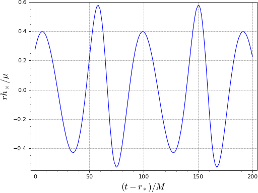
A plot of the waveform generated by a particle orbiting at the ISCO:

sage: hc = lambda u: h_cross_particle(a, 6., u, pi/4, 0.)
sage: plot(hc, (0, 200.), axes_labels=[r'$(t-r_*)/M$', r'$r h_\times/\mu$'],
....:      gridlines=True, frame=True, axes=False)
Graphics object consisting of 1 graphics primitive

Case \(a/M=0.95\) (rapidly rotating Kerr black hole):

sage: a = 0.95
sage: h_cross_particle(a, 2., 0., pi/4, 0.)  # tol 1.0e-13
-0.2681353673743396

Assessing the importance of the mode \(m=1\):

sage: h_cross_particle(a, 2., 0., pi/4, 0., m_min=2)  # tol 1.0e-13
-0.3010579420748449

kerrgeodesic_gw.gw_particle.h_cross_particle_fourier(m, a, r0, theta, l_max=10, algorithm_Zinf='spline')

Return the Fourier mode of a given order \(m\) of the rescaled \(h_\times\)-part of the gravitational wave emitted by a particle in circular orbit around a Kerr black hole.

The rescaled Fourier mode of order \(m\) received at the location \((t,r,\theta,\phi)\) is

\[\frac{r}{\mu} h_m^\times = {\bar A}_m^\times \cos(m\psi) + {\bar B}_m^\times \sin(m\psi)\]

where \(\mu\) is the particle mass and \(\psi := \omega_0 (t-r_*) - \phi\), \(\omega_0\) being the orbital frequency of the particle and \(r_*\) the tortoise coordinate corresponding to \(r\) and \({\bar A}_m^\times\) and \({\bar B}_m^\times\) are given by Eqs. (5)-(6) above.

INPUT:

• m – positive integer defining the Fourier mode

• a – BH angular momentum parameter (in units of \(M\), the BH mass)

• r0 – Boyer-Lindquist radius of the orbit (in units of \(M\))

• theta – Boyer-Lindquist colatitute \(\theta\) of the observer

• l_max – (default: 10) upper bound in the summation over the harmonic degree \(\ell\) in Eqs. (5)-(6)

• algorithm_Zinf – (default: 'spline') string describing the computational method for \(Z^\infty_{\ell m}(r_0)\); allowed values are

  • 'spline': spline interpolation of tabulated data

  • '1.5PN' (only for a=0): 1.5-post-Newtonian expansion following E. Poisson, Phys. Rev. D 47, 1497 (1993) [doi:10.1103/PhysRevD.47.1497]

OUTPUT:

• tuple \(({\bar A}_m^\times, {\bar B}_m^\times)\)

EXAMPLES:

Let us consider the case \(a=0\) first (Schwarzschild black hole), with \(m=2\):

sage: from kerrgeodesic_gw import h_cross_particle_fourier
sage: a = 0

\(h_m^\times\) is always zero in the direction \(\theta=\pi/2\):

sage: h_cross_particle_fourier(2, a, 8., pi/2)  # tol 1.0e-13
(3.444996575846961e-17, 1.118234985040581e-16)

Let us then evaluate \(h_m^\times\) in the direction \(\theta=\pi/4\):

sage: h_cross_particle_fourier(2, a, 8., pi/4)  # tol 1.0e-13
(0.09841144532628172, 0.31201728756415015)
sage: h_cross_particle_fourier(2, a, 8., pi/4, l_max=5)  # tol 1.0e-13
(0.09841373523119075, 0.31202073689061305)
sage: h_cross_particle_fourier(2, a, 8., pi/4, l_max=5, algorithm_Zinf='1.5PN')  # tol 1.0e-13
(0.11744823578781578, 0.34124272645755677)

Values of \(m\) different from 2:

sage: h_cross_particle_fourier(3, a, 20., pi/4)  # tol 1.0e-13
(0.022251439699635174, -0.005354134279052387)
sage: h_cross_particle_fourier(3, a, 20., pi/4, l_max=5, algorithm_Zinf='1.5PN')  # tol 1.0e-13
(0.017782177999686274, 0.0)
sage: h_cross_particle_fourier(1, a, 8., pi/4)  # tol 1.0e-13
(0.03362589948237155, -0.008465651545641889)
sage: h_cross_particle_fourier(0, a, 8., pi/4)
(0, 0)

The case \(a/M=0.95\) (rapidly rotating Kerr black hole):

sage: a = 0.95
sage: h_cross_particle_fourier(2, a, 8., pi/4)  # tol 1.0e-13
(0.08843838892991202, 0.28159329265206867)
sage: h_cross_particle_fourier(8, a, 8., pi/4)  # tol 1.0e-13
(-0.00014588821622195107, -8.179557811364057e-06)
sage: h_cross_particle_fourier(2, a, 2., pi/4)  # tol 1.0e-13
(-0.6021994882885746, 0.3789513303450391)
sage: h_cross_particle_fourier(8, a, 2., pi/4)  # tol 1.0e-13
(0.01045760329050054, -0.004986913120370192)

kerrgeodesic_gw.gw_particle.h_particle_quadrupole(r0, u, theta, phi, phi0=0, mode='+')

Return the rescaled \(h_+\) or \(h_\times\) part of the gravitational radiation emitted by a particle in quasi-Newtonian circular orbit around a massive body, computed at the quadrupole approximation.

The computation is performed according to the following formulas:

\[\begin{split}\begin{array}{l} \displaystyle h_+ = 2\, \frac{\mu}{r} \frac{M}{r_0} (1+\cos^2\theta) \cos\left[2\omega_0 (t - r) + 2(\phi_0-\phi)\right] \\ \displaystyle h_\times = 4\, \frac{\mu}{r} \frac{M}{r_0} \cos\theta \sin\left[2\omega_0 (t - r) + 2(\phi_0-\phi)\right] \end{array}\end{split}\]

where \(M\) is the mass of the central body, \(\mu\ll M\) the mass of the orbiting particle, \(r_0\) the orbital radius, \(\omega_0 = \sqrt{M/r_0^3}\) the corresponding orbital angular velocity and \((t, r, \theta,\phi)\) the coordinates of the observer.

INPUT:

• r0 – radius of the orbit (in units of \(M\), the mass of the central body)

• u – retarded time coordinate \(u = t - r\) of the observer (in units of \(M\))

• theta – colatitute \(\theta\) of the observer

• phi – azimuthal coordinate \(\phi\) of the observer

• phi0 – (default: 0) phase factor

• mode – (default: '+') string determining which GW polarization mode is considered; allowed values are '+' and 'x', for respectively \(h_+\) and \(h_\times\)

OUTPUT:

• the rescaled waveform \((r / \mu) h\), where \(\mu\) is the particle’s mass, \(r\) is the radial coordinate of the observer and \(h\) is either \(h_+\) or \(h_\times\) (depending on the value of mode)

EXAMPLES:

Values of \(h_+\) for \(r_0 = 12 M\):

sage: from kerrgeodesic_gw import (h_particle_quadrupole,
....:                              h_plus_particle, h_cross_particle)
sage: theta, phi = pi/3, 0
sage: r0 = 12.
sage: porb = n(2*pi*r0^1.5)  # orbital period
sage: u = porb/16
sage: h_particle_quadrupole(r0, u, theta, phi)  # tol 1.0e-13
0.1473139127471974
sage: h_plus_particle(0., r0, u, theta, phi)  # exact value, tol 1.0e-13
0.041745779012809306
sage: h_plus_particle(0., r0, u, theta, phi, l_max=5,
....:                 algorithm_Zinf='1.5PN')  # 1.5 PN approx, tol 1.0e-13
0.06396788402755646

Values of \(h_\times\) for \(r_0 = 12 M\):

sage: h_particle_quadrupole(r0, u, theta, phi, mode='x')  # tol 1.0e-13
0.1178511301977579
sage: h_cross_particle(0., r0, u, theta, phi)  # exact value, tol 1.0e-13
0.1351232731503482
sage: h_cross_particle(0., r0, u, theta, phi, l_max=5,
....:                  algorithm_Zinf='1.5PN')  # 1.5 PN approx, tol 1.0e-13
0.14924631043762673

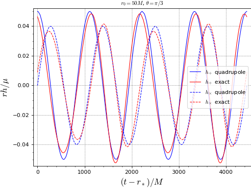
Values of \(h_+\) for \(r_0 = 50 M\):

sage: r0 = 50.
sage: porb = n(2*pi*r0^1.5)  # orbital period
sage: u = porb/16
sage: h_particle_quadrupole(r0, u, theta, phi)  # tol 1.0e-13
0.03535533905932738
sage: h_plus_particle(0., r0, u, theta, phi, l_max=5)  # exact value, tol 1.0e-13
0.024850367000986223
sage: h_plus_particle(0., r0, u, theta, phi, l_max=5,
....:                 algorithm_Zinf='1.5PN')  # 1.5 PN approx, tol 1.0e-13
0.026007035506911764

The difference between the exact value and the one resulting from the quadrupole approximation looks large, but actually this results mostly from some dephasing, as one can see on a plot:

sage: hp_quad = lambda t: h_particle_quadrupole(r0, t, theta, phi)
sage: hc_quad = lambda t: h_particle_quadrupole(r0, t, theta, phi, mode='x')
sage: hp = lambda t: h_plus_particle(0., r0, t, theta, phi, l_max=5)
sage: hc = lambda t: h_cross_particle(0., r0, t, theta, phi, l_max=5)
sage: umax = 2*porb
sage: plot(hp_quad, (0, umax), legend_label=r'$h_+$ quadrupole',
....:      axes_labels=[r'$(t-r_*)/M$', r'$r h/\mu$'],
....:      title=r'$r_0=50 M$, $\theta=\pi/3$',
....:      gridlines=True, frame=True, axes=False) + \
....: plot(hp, (0, umax), color='red', legend_label=r'$h_+$ exact') + \
....: plot(hc_quad, (0, umax), linestyle='--',
....:      legend_label=r'$h_\times$ quadrupole') + \
....: plot(hc, (0, umax), color='red', linestyle='--',
....:      legend_label=r'$h_\times$ exact')
Graphics object consisting of 4 graphics primitives

kerrgeodesic_gw.gw_particle.h_particle_signal(a, r0, theta, phi, u_min, u_max, mode='+', nb_points=100, phi0=0, l_max=10, m_min=1, approximation=None, store=None)

Return a time sequence of the \(h_+\) or the \(h_\times\) part of the gravitational radiation from a particle in circular orbit around a Kerr black hole.

Note

It is more efficient to use this function than to perform a loop over h_plus_particle() or h_cross_particle(). Indeed, the Fourier modes, which involve the computation of spin-weighted spheroidal harmonics and of the functions \(Z^\infty_{\ell m}(r_0)\), are evaluated once for all, prior to the loop on the retarded time \(u\).

INPUT:

• a – BH angular momentum parameter (in units of \(M\))

• r0 – Boyer-Lindquist radius of the orbit (in units of \(M\))

• theta – Boyer-Lindquist colatitute \(\theta\) of the observer

• phi – Boyer-Lindquist azimuthal coordinate \(\phi\) of the observer

• u_min – lower bound of the retarded time coordinate of the observer (in units of the black hole mass \(M\)): \(u = t - r_*\), where \(t\) is the Boyer-Lindquist time coordinate and \(r_*\) is the tortoise coordinate

• u_max – upper bound of the retarded time coordinate of the observer (in units of the black hole mass \(M\))

• mode – (default: '+') string determining which GW polarization mode is considered; allowed values are '+' and 'x', for respectively \(h_+\) and \(h_\times\)

• nb_points – (default: 100) number of points in the interval (u_min, u_max)

• phi0 – (default: 0) phase factor

• l_max – (default: 10) upper bound in the summation over the harmonic degree \(\ell\)

• m_min – (default: 1) lower bound in the summation over the Fourier mode \(m\)

• approximation – (default: None) string describing the computational method; allowed values are

  • None: exact computation

  • '1.5PN' (only for a=0): 1.5-post-Newtonian expansion following E. Poisson, Phys. Rev. D 47, 1497 (1993) [doi:10.1103/PhysRevD.47.1497]

  • 'quadrupole' (only for a=0): quadrupole approximation (0-post-Newtonian); see h_particle_quadrupole()

• store – (default: None) string containing a file name for storing the time sequence; if None, no storage is attempted

OUTPUT:

• a list of nb_points pairs \((u, r h/\mu)\), where \(u\) is the retarded time, \(h\) is either \(h_+\) or \(h_\times\) depending on the parameter mode, \(\mu\) is the particle mass and \(r\) is the Boyer-Lindquist radial coordinate of the observer

EXAMPLES:

\(h_+\) signal at \(\theta=\pi/2\) from a particle at the ISCO of a Schwarzschild black hole (\(a=0\), \(r_0=6M\)):

sage: from kerrgeodesic_gw import h_particle_signal
sage: h_particle_signal(0., 6., pi/2, 0., 0., 200., nb_points=9)  # tol 1.0e-13
[(0.000000000000000, 0.1536656546005028),
 (25.0000000000000, -0.2725878162016865),
 (50.0000000000000, 0.3525164756465054),
 (75.0000000000000, 0.047367530900643974),
 (100.000000000000, -0.06816472285771447),
 (125.000000000000, -0.10904082076122341),
 (150.000000000000, 0.11251491162759894),
 (175.000000000000, 0.2819301792449237),
 (200.000000000000, -0.24646401049292863)]

Storing the sequence in a file:

sage: h = h_particle_signal(0., 6., pi/2, 0., 0., 200.,
....:                       nb_points=9, store='h_plus.d')

The \(h_\times\) signal, for \(\theta=\pi/4\):

sage: h_particle_signal(0., 6., pi/4, 0., 0., 200., nb_points=9, mode='x')  # tol 1.0e-13
[(0.000000000000000, 0.275027796440582),
 (25.0000000000000, -0.18713017721920192),
 (50.0000000000000, 0.2133141583155321),
 (75.0000000000000, -0.531073507307601),
 (100.000000000000, 0.3968872953624949),
 (125.000000000000, -0.4154274307718398),
 (150.000000000000, 0.5790969355083798),
 (175.000000000000, -0.24074783639714234),
 (200.000000000000, 0.22869838143661578)]

kerrgeodesic_gw.gw_particle.h_plus_particle(a, r0, u, theta, phi, phi0=0, l_max=10, m_min=1, algorithm_Zinf='spline')

Return the rescaled \(h_+\)-part of the gravitational radiation emitted by a particle in circular orbit around a Kerr black hole.

The computation is based on Eq. (2) above.

INPUT:

• a – BH angular momentum parameter (in units of \(M\), the BH mass)

• r0 – Boyer-Lindquist radius of the orbit (in units of \(M\))

• u – retarded time coordinate of the observer (in units of \(M\)): \(u = t - r_*\), where \(t\) is the Boyer-Lindquist time coordinate and \(r_*\) is the tortoise coordinate

• theta – Boyer-Lindquist colatitute \(\theta\) of the observer

• phi – Boyer-Lindquist azimuthal coordinate \(\phi\) of the observer

• phi0 – (default: 0) phase factor

• l_max – (default: 10) upper bound in the summation over the harmonic degree \(\ell\)

• m_min – (default: 1) lower bound in the summation over the Fourier mode \(m\)

• algorithm_Zinf – (default: 'spline') string describing the computational method for \(Z^\infty_{\ell m}(r_0)\); allowed values are

  • 'spline': spline interpolation of tabulated data

  • '1.5PN' (only for a=0): 1.5-post-Newtonian expansion following E. Poisson, Phys. Rev. D 47, 1497 (1993) [doi:10.1103/PhysRevD.47.1497]

OUTPUT:

• the rescaled waveform \((r / \mu) h_+\), where \(\mu\) is the particle’s mass and \(r\) is the Boyer-Lindquist radial coordinate of the observer

EXAMPLES:

Let us consider the case \(a=0\) (Schwarzschild black hole) and \(r_0=6 M\) (emission from the ISCO):

sage: from kerrgeodesic_gw import h_plus_particle
sage: a = 0
sage: h_plus_particle(a, 6., 0., pi/2, 0.)  # tol 1.0e-13
0.1536656546005028
sage: h_plus_particle(a, 6., 0., pi/2, 0., l_max=5)  # tol 1.0e-13
0.157759938177291
sage: h_plus_particle(a, 6., 0., pi/2, 0., l_max=5, algorithm_Zinf='1.5PN')  # tol 1.0e-13
0.22583887001798497

For an orbit of larger radius (\(r_0=12 M\)), the 1.5-post-Newtonian approximation is in better agreement with the exact computation:

sage: h_plus_particle(a, 12., 0., pi/2, 0.)  # tol 1.0e-13
0.11031251832047866
sage: h_plus_particle(a, 12., 0., pi/2, 0., l_max=5, algorithm_Zinf='1.5PN')  # tol 1.0e-13
0.12935832450325302

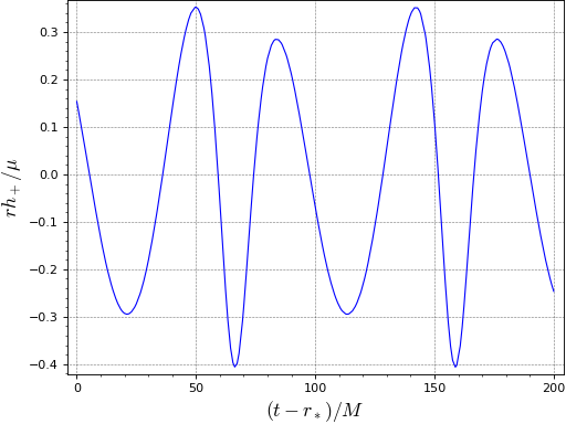
A plot of the waveform generated by a particle orbiting at the ISCO:

sage: hp = lambda u: h_plus_particle(a, 6., u, pi/2, 0.)
sage: plot(hp, (0, 200.), axes_labels=[r'$(t-r_*)/M$', r'$r h_+/\mu$'],
....:      gridlines=True, frame=True, axes=False)
Graphics object consisting of 1 graphics primitive

Case \(a/M=0.95\) (rapidly rotating Kerr black hole):

sage: a = 0.95
sage: h_plus_particle(a, 2., 0., pi/2, 0.)  # tol 1.0e-13
0.20326150400852214

Assessing the importance of the mode \(m=1\):

sage: h_plus_particle(a, 2., 0., pi/2, 0., m_min=2)  # tol 1.0e-13
0.21845811047370495

kerrgeodesic_gw.gw_particle.h_plus_particle_fourier(m, a, r0, theta, l_max=10, algorithm_Zinf='spline')

Return the Fourier mode of a given order \(m\) of the rescaled \(h_+\)-part of the gravitational wave emitted by a particle in circular orbit around a Kerr black hole.

The rescaled Fourier mode of order \(m\) received at the location \((t,r,\theta,\phi)\) is

\[\frac{r}{\mu} h_m^+ = {\bar A}_m^+ \cos(m\psi) + {\bar B}_m^+ \sin(m\psi)\]

where \(\mu\) is the particle mass and \(\psi := \omega_0 (t-r_*) - \phi\), \(\omega_0\) being the orbital frequency of the particle and \(r_*\) the tortoise coordinate corresponding to \(r\) and \({\bar A}_m^+\) and \({\bar B}_m^+\) are given by Eqs. (3)-(4) above.

INPUT:

• m – positive integer defining the Fourier mode

• a – BH angular momentum parameter (in units of \(M\), the BH mass)

• r0 – Boyer-Lindquist radius of the orbit (in units of \(M\))

• theta – Boyer-Lindquist colatitute \(\theta\) of the observer

• l_max – (default: 10) upper bound in the summation over the harmonic degree \(\ell\) in Eqs. (3)-(4)

• algorithm_Zinf – (default: 'spline') string describing the computational method for \(Z^\infty_{\ell m}(r_0)\); allowed values are

  • 'spline': spline interpolation of tabulated data

  • '1.5PN' (only for a=0): 1.5-post-Newtonian expansion following E. Poisson, Phys. Rev. D 47, 1497 (1993) [doi:10.1103/PhysRevD.47.1497]

OUTPUT:

• tuple \(({\bar A}_m^+, {\bar B}_m^+)\)

EXAMPLES:

Let us consider the case \(a=0\) first (Schwarzschild black hole), with \(m=2\):

sage: from kerrgeodesic_gw import h_plus_particle_fourier
sage: a = 0
sage: h_plus_particle_fourier(2, a, 8., pi/2)  # tol 1.0e-13
(0.2014580652208302, -0.06049343736886148)
sage: h_plus_particle_fourier(2, a, 8., pi/2, l_max=5)  # tol 1.0e-13
(0.20146097329552273, -0.060495372034569186)
sage: h_plus_particle_fourier(2, a, 8., pi/2, l_max=5, algorithm_Zinf='1.5PN')  # tol 1.0e-13
(0.2204617125753912, -0.0830484439639611)

Values of \(m\) different from 2:

sage: h_plus_particle_fourier(3, a, 20., pi/2)  # tol 1.0e-13
(-0.005101595598729037, -0.021302121442654077)
sage: h_plus_particle_fourier(3, a, 20., pi/2, l_max=5, algorithm_Zinf='1.5PN')  # tol 1.0e-13
(0.0, -0.016720919174427588)
sage: h_plus_particle_fourier(1, a, 8., pi/2)  # tol 1.0e-13
(-0.014348477201223874, -0.05844679575244101)
sage: h_plus_particle_fourier(0, a, 8., pi/2)
(0, 0)

The case \(a/M=0.95\) (rapidly rotating Kerr black hole):

sage: a = 0.95
sage: h_plus_particle_fourier(2, a, 8., pi/2)  # tol 1.0e-13
(0.182748773431646, -0.05615306925896938)
sage: h_plus_particle_fourier(8, a, 8., pi/2)  # tol 1.0e-13
(-4.724709221209198e-05, 0.0006867183495228116)
sage: h_plus_particle_fourier(2, a, 2., pi/2)  # tol 1.0e-13
(0.1700402877617014, 0.33693580916655747)
sage: h_plus_particle_fourier(8, a, 2., pi/2)  # tol 1.0e-13
(-0.009367442995129153, -0.03555092085651877)

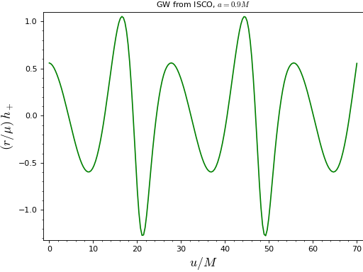
kerrgeodesic_gw.gw_particle.plot_h_particle(a, r0, theta, phi, u_min, u_max, plot_points=200, phi0=0, l_max=10, m_min=1, approximation=None, mode=('+', 'x'), color=None, linestyle=None, legend_label=('$h_+$', '$h_\\\\times$'), xlabel='$(t - r_*)/M$', ylabel=None, title=None, gridlines=True)

Plot the gravitational waveform emitted by a particle in circular orbit around a Kerr black hole.

INPUT:

• a – BH angular momentum parameter (in units of \(M\), the black hole mass)

• r0 – Boyer-Lindquist radius of the orbit (in units of \(M\))

• theta – Boyer-Lindquist colatitute \(\theta\) of the observer

• phi – Boyer-Lindquist azimuthal coordinate \(\phi\) of the observer

• u_min – lower bound of the retarded time coordinate of the observer (in units of \(M\)): \(u = t - r_*\), where \(t\) is the Boyer-Lindquist time coordinate and \(r_*\) is the tortoise coordinate

• u_max – upper bound of the retarded time coordinate of the observer (in units of \(M\))

• plot_points – (default: 200) number of points involved in the sampling of the interval (u_min, u_max)

• phi0 – (default: 0) phase factor

• l_max – (default: 10) upper bound in the summation over the harmonic degree \(\ell\)

• m_min – (default: 1) lower bound in the summation over the Fourier mode \(m\)

• approximation – (default: None) string describing the computational method; allowed values are

  • None: exact computation

  • '1.5PN' (only for a=0): 1.5-post-Newtonian expansion following E. Poisson, Phys. Rev. D 47, 1497 (1993) [doi:10.1103/PhysRevD.47.1497]

  • 'quadrupole' (only for a=0): quadrupole approximation (0-post-Newtonian); see h_particle_quadrupole()

• mode – (default: ('+', 'x')) string determining the plotted quantities: allowed values are '+' and 'x', for respectively \(h_+\) and \(h_\times\), as well as ('+', 'x') for plotting both polarization modes

• color – (default: None) a color (if mode = '+' or 'x') or a pair of colors (if mode = ('+', 'x')) for the plot(s); if None, the default colors are 'blue' for \(h_+\) and 'red' for \(h_\times\)

• linestyle – (default: None) a line style (if mode = '+' or 'x') or a pair of line styles (if mode = ('+', 'x')) for the plot(s); if None, the default style is a solid line

• legend_label – (default: (r'$h_+$', r'$h_\times$')) labels for the plots of \(h_+\) and \(h_\times\); used only if mode is ('+', 'x')

• xlabel – (default: r'$(t - r_*)/M$') label of the \(x\)-axis

• ylabel – (default: None) label of the \(y\)-axis; if None, r'$(r/\mu)\, h_+$' is used for mode = '+', r'$(r/\mu)\, h_\times$' for mode = 'x' and r'$(r/\mu)\, h_{+,\times}$' for mode = ('+', 'x')

• title – (default: None) plot title; if None, the title is generated from a, r0 and theta (see the example below)

• gridlines – (default: True) indicates whether the gridlines are to be plotted

OUTPUT:

• a graphics object

EXAMPLES:

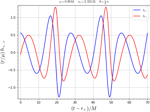
Plot of the gravitational waveform generated by a particle orbiting at the ISCO of a Kerr black hole with \(a=0.9 M\):

sage: from kerrgeodesic_gw import plot_h_particle
sage: plot_h_particle(0.9, 2.321, pi/4, 0., 0., 70.)
Graphics object consisting of 2 graphics primitives

Plot of \(h_+\) only, with some non-default options:

sage: plot_h_particle(0.9, 2.321, pi/4, 0., 0., 70., mode='+',
....:                 color='green', xlabel=r'$u/M$', gridlines=False,
....:                 title='GW from ISCO, $a=0.9M$')
Graphics object consisting of 1 graphics primitive

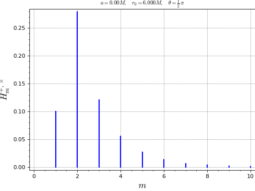
kerrgeodesic_gw.gw_particle.plot_spectrum_particle(a, r0, theta, mode='+', m_max=10, l_max=10, algorithm_Zinf='spline', color='blue', linestyle='-', thickness=2, legend_label=None, offset=0, xlabel=None, ylabel=None, title=None, gridlines=True)

Plot the Fourier spectrum of the gravitational radiation emitted by a particle in equatorial circular orbit around a Kerr black hole.

The Fourier spectrum is defined by the following sequence indexed by \(m\):

\[H^{+,\times}_m(\theta) := \frac{r}{\mu} \sqrt{(A_m^{+,\times}(\theta))^2 + (B_m^{+,\times}(\theta))^2}\]

where the functions \(A_m^+\), \(B_m^+\), \(A_m^\times\), \(B_m^\times\) are defined by (2).

INPUT:

• a – BH angular momentum parameter (in units of \(M\), the BH mass)

• r0 – Boyer-Lindquist radius of the orbit (in units of \(M\))

• theta – Boyer-Lindquist colatitute \(\theta\) of the observer

• mode – (default: '+') string determining which GW polarization mode is considered; allowed values are '+' and 'x', for respectively \(h_+\) and \(h_\times\)

• m_max – (default: 10) maximal value of \(m\)

• l_max – (default: 10) upper bound in the summation over the harmonic degree \(\ell\)

• algorithm_Zinf – (default: 'spline') string describing the computational method for \(Z^\infty_{\ell m}(r_0)\); allowed values are

  • 'spline': spline interpolation of tabulated data

  • '1.5PN' (only for a=0): 1.5-post-Newtonian expansion following E. Poisson, Phys. Rev. D 47, 1497 (1993) [doi:10.1103/PhysRevD.47.1497]

• color – (default: 'blue') color of vertical lines

• linestyle – (default: '-') style of vertical lines

• legend_label – (default: None) legend label for this spectrum

• offset – (default: 0) horizontal offset for the position of the vertical lines

• xlabel – (default: None) label of the x-axis; if none is provided, the label is set to \(m\)

• ylabel – (default: None) label of the y-axis; if none is provided, the label is set to \(H_m^{+,\times}\)

• title – (default: None) plot title; if None, the title is generated from a, r0 and theta

• gridlines – (default: True) indicates whether the gridlines are to be plotted

OUTPUT:

• a graphics object

EXAMPLES:

Spectrum of gravitational radiation generated by a particle orbiting at the ISCO of a Schwarzschild black hole (\(a=0\), \(r_0=6M\)):

sage: from kerrgeodesic_gw import plot_spectrum_particle
sage: plot_spectrum_particle(0, 6., pi/2)
Graphics object consisting of 10 graphics primitives

kerrgeodesic_gw.gw_particle.radiated_power_particle(a, r0, l_max=None, m_min=1, approximation=None)

Return the total (i.e. summed over all directions) power of the gravitational radiation emitted by a particle in circular orbit around a Kerr black hole.

The total radiated power (or luminosity) \(L\) is computed according to the formula:

\[L = \frac{\mu^2}{4\pi} \sum_{\ell=2}^{\infty} \sum_{{\scriptstyle m=-\ell\atop \scriptstyle m\not=0}}^\ell \frac{\left| Z^\infty_{\ell m}(r_0) \right| ^2}{(m\omega_0)^2}\]

INPUT:

• a – BH angular momentum parameter (in units of \(M\), the BH mass)

• r0 – Boyer-Lindquist radius of the orbit (in units of \(M\))

• l_max – (default: None) upper bound in the summation over the harmonic degree \(\ell\); if None, l_max is determined automatically from the available tabulated data

• m_min – (default: 1) lower bound in the summation over the Fourier mode \(m\)

• approximation – (default: None) string describing the computational method; allowed values are

  • None: exact computation

  • '1.5PN' (only for a=0): 1.5-post-Newtonian expansion following E. Poisson, Phys. Rev. D 47, 1497 (1993) [doi:10.1103/PhysRevD.47.1497]

  • 'quadrupole' (only for a=0): quadrupole approximation (0-post-Newtonian); see h_particle_quadrupole()

OUTPUT:

• rescaled radiated power \(L\, (M/\mu)^2\), where \(M\) is the BH mass and \(\mu\) the mass of the orbiting particle.

EXAMPLES:

Power radiated by a particle at the ISCO of a Schwarzschild BH:

sage: from kerrgeodesic_gw import radiated_power_particle
sage: radiated_power_particle(0, 6.)
0.000937262782177525

Power radiated by a particle at the ISCO of a rapidly rotating Kerr BH (\(a=0.98 M\)):

sage: radiated_power_particle(0.98, 1.61403)  # tol 1.0e-13
0.08629927053494096

Power computed according to various approximations:

sage: radiated_power_particle(0, 6., approximation='1.5PN')  # tol 1.0e-13
0.0010435864384751143
sage: radiated_power_particle(0, 6., approximation='quadrupole')  # tol 1.0e-13
0.000823045267489712

Let us check that at large radius, these approximations get closer to the actual result:

sage: radiated_power_particle(0, 50.)  # tol 1.0e-13
1.9624555021692417e-08
sage: radiated_power_particle(0, 50., approximation='1.5PN')  # tol 1.0e-13
1.958318200436188e-08
sage: radiated_power_particle(0, 50., approximation='quadrupole')  # tol 1.0e-13
2.0480000000000002e-08

kerrgeodesic_gw.gw_particle.secular_frequency_change(a, r0, l_max=None, m_min=1, approximation=None)

Return the gravitational-radiation induced change of the orbital frequency of a particle in circular orbit around a Kerr black hole.

INPUT:

• a – BH angular momentum parameter (in units of \(M\), the BH mass)

• r0 – Boyer-Lindquist radius of the orbit (in units of \(M\))

• l_max – (default: None) upper bound in the summation over the harmonic degree \(\ell\); if None, l_max is determined automatically from the available tabulated data

• m_min – (default: 1) lower bound in the summation over the Fourier mode \(m\)

• approximation – (default: None) string describing the computational method; allowed values are

  • None: exact computation

  • '1.5PN' (only for a=0): 1.5-post-Newtonian expansion following E. Poisson, Phys. Rev. D 47, 1497 (1993) [doi:10.1103/PhysRevD.47.1497]

  • 'quadrupole' (only for a=0): quadrupole approximation (0-post-Newtonian); see h_particle_quadrupole()

OUTPUT:

• rescaled fractional change in orbital frequency \(\dot{\omega}_0/\omega_0 \, (M^2/\mu)\), where \(M\) is the BH mass and \(\mu\) the mass of the orbiting particle.

EXAMPLES:

Relative change in orbital frequency change at \(r_0 = 10 M\) around a Schwarzschild black hole:

sage: from kerrgeodesic_gw import secular_frequency_change
sage: secular_frequency_change(0, 10)  # tol 1.0e-13
0.002701529506901975
sage: secular_frequency_change(0, 10, approximation='quadrupole')  # tol 1.0e-13
0.00192

At larger distance, the quadrupole approximation works better:

sage: secular_frequency_change(0, 50)  # tol 1.0e-13
3.048598175592674e-06
sage: secular_frequency_change(0, 50, approximation='quadrupole')  # tol 1.0e-13
3.072e-06

At the ISCO, \(\dot{\omega}_0\) diverges:

sage: secular_frequency_change(0, 6)
+infinity

while the quadrupole approximation would have predict a finite value there:

sage: secular_frequency_change(0, 6, approximation='quadrupole')  # tol 1.0e-13
0.014814814814814817

Case of a Kerr black hole:

sage: secular_frequency_change(0.5, 6)  # tol 1.0e-13
0.020393023677356764