Signal processing

Signal processing

kerrgeodesic_gw.signal_processing.fourier(signal)

Compute the Fourier transform of a time signal.

The Fourier transform of the time signal \(h(t)\) is defined by

\[\tilde{h}(f) = \int_{-\infty}^{+\infty} h(t)\, \mathrm{e}^{-2\pi \mathrm{i} f t} \, \mathrm{d}t\]

INPUT:

• signal – list of pairs \((t, h(t))\), where \(t\) is the time and \(h(t)\) is the signal at \(t\). NB: the sampling in \(t\) must be uniform

OUTPUT:

• a numerical approximation (FFT) of the Fourier transform, as a list of pairs \((f,\tilde{h}(f))\)

EXAMPLES:

Fourier transform of the \(h_+\) signal from a particle orbiting at the ISCO of a Schwarzschild black hole:

sage: from kerrgeodesic_gw import h_particle_signal, fourier
sage: a, r0 = 0., 6.
sage: theta, phi = pi/2, 0
sage: sig = h_particle_signal(a, r0, theta, phi, 0., 800., nb_points=200)
sage: sig[:5]  # tol 1.0e-13
[(0.000000000000000, 0.1536656546005028),
 (4.02010050251256, 0.03882960191740132),
 (8.04020100502512, -0.0791773803745108),
 (12.0603015075377, -0.18368354016995483),
 (16.0804020100502, -0.25796165580196795)]
sage: ft = fourier(sig)
sage: ft[:5]   # tol 1.0e-13
[(-0.12437500000000001, (1.0901773159466113+0j)),
 (-0.12313125000000001, (1.0901679813096925+0.021913447210468399j)),
 (-0.12188750000000001, (1.0901408521337845+0.043865034665617614j)),
 (-0.12064375000000001, (1.0900987733011678+0.065894415355341171j)),
 (-0.11940000000000001, (1.0900473072498438+0.088044567109304195j))]

Plot of the norm of the Fourier transform:

sage: ft_norm = [(f, abs(hf)) for (f, hf) in ft]
sage: line(ft_norm, axes_labels=[r'$f M$', r'$|\tilde{h}_+(f)| r/(\mu M)$'],
....:      gridlines=True, frame=True, axes=False)
Graphics object consisting of 1 graphics primitive

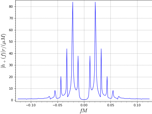
The first peak is at the orbital frequency of the particle:

sage: f0 = n(1/(2*pi*r0^(3/2))); f0
0.0108291222393566

while the highest peak is at twice this frequency (\(m=2\) mode).

kerrgeodesic_gw.signal_processing.max_detectable_radius(a, mu, theta, psd, BH_time_scale, distance, t_obs_yr=1, snr_threshold=10, r_min=None, r_max=200, m_min=1, m_max=None, approximation=None)

Compute the maximum orbital radius \(r_{0,\rm max}\) at which a particle of given mass is detectable.

INPUT:

• a – BH angular momentum parameter (in units of \(M\), the BH mass)

• mu – mass of the orbiting object, in solar masses

• theta – Boyer-Lindquist colatitute \(\theta\) of the observer

• psd – function with a single argument (\(f\)) representing the detector’s one-sided noise power spectral density \(S_n(f)\) (see e.g. lisa_detector.power_spectral_density())

• BH_time_scale – value of \(M\) in the same time unit as \(S_n(f)\); if \(S_n(f)\) is provided in \(\mathrm{Hz}^{-1}\), then BH_time_scale must be \(M\) expressed in seconds.

• distance – distance \(r\) to the detector, in parsecs

• t_obs_yr – (default: 1) observation period, in years

• snr_threshold – (default: 10) signal-to-noise value above which a detection is claimed

• r_min – (default: None) lower bound of the search interval for \(r_{0,\rm max}\) (in units of \(M\)); if None then the ISCO value is used

• r_max – (default: 200) upper bound of the search interval for \(r_{0,\rm max}\) (in units of \(M\))

• m_min – (default: 1) lower bound in the summation over the Fourier mode \(m\)

• m_max – (default: None) upper bound in the summation over the Fourier mode \(m\); if None, m_max is set to 10 for \(r_0 \leq 20 M\) and to 5 for \(r_0 > 20 M\)

• approximation – (default: None) string describing the computational method for the signal; allowed values are

  • None: exact computation

  • 'quadrupole': quadrupole approximation; see gw_particle.h_particle_quadrupole()

  • '1.5PN' (only for a=0): 1.5-post-Newtonian expansion following E. Poisson, Phys. Rev. D 47, 1497 (1993) [doi:10.1103/PhysRevD.47.1497]

OUTPUT:

• Boyer-Lindquist radius (in units of \(M\)) of the most remote orbit for which the signal-to-noise ratio is larger than snr_threshold during the observation time t_obs_yr

EXAMPLES:

Maximum orbital radius for LISA detection of a 1 solar-mass object orbiting Sgr A* observed by LISA, assuming a BH spin \(a=0.9 M\) and a vanishing inclination angle:

sage: from kerrgeodesic_gw import (max_detectable_radius, lisa_detector,
....:                              astro_data)
sage: a = 0.9
sage: mu = 1
sage: theta = 0
sage: psd = lisa_detector.power_spectral_density_RCLfit
sage: BH_time_scale = astro_data.SgrA_mass_s
sage: distance = astro_data.SgrA_distance_pc
sage: max_detectable_radius(a, mu, theta, psd, BH_time_scale, distance)  # tol 1.0e-13
46.98292057022975

Lowering the SNR threshold to 5:

sage: max_detectable_radius(a, mu, theta, psd, BH_time_scale, distance,  # tol 1.0e-13
....:                       snr_threshold=5)
53.503386416644645

Lowering the data acquisition time to 1 day:

sage: max_detectable_radius(a, mu, theta, psd, BH_time_scale, distance,  # tol 1.0e-13
....:                       t_obs_yr=1./365.25)
27.158725683511463

Assuming an inclination angle of \(\pi/2\):

sage: theta = pi/2
sage: max_detectable_radius(a, mu, theta, psd, BH_time_scale, distance)  # tol 1.0e-13
39.81826500968452

Using the 1.5-PN approximation (a has to be zero and m_max has to be at most 5):

sage: a = 0
sage: max_detectable_radius(a, mu, theta, psd, BH_time_scale,  # tol 1.0e-13
....:                       distance, approximation='1.5PN', m_max=5)
39.74273792957649

kerrgeodesic_gw.signal_processing.read_signal(filename, dirname=None)

Read a signal from a data file.

INPUT:

• filename – string; name of the file

• dirname – (default: None) string; name of directory where the file is located

OUTPUT:

• signal as a list of pairs \((t, h(t))\)

EXAMPLES:

sage: from kerrgeodesic_gw import save_signal, read_signal
sage: sig0 = [(RDF(i/10), RDF(sin(i/5))) for i in range(5)]
sage: from sage.misc.temporary_file import tmp_filename
sage: filename = tmp_filename(ext='.dat')
sage: save_signal(sig0, filename)
sage: sig = read_signal(filename)
sage: sig   # tol 1.0e-13
[(0.0, 0.0),
 (0.1, 0.19866933079506122),
 (0.2, 0.3894183423086505),
 (0.3, 0.5646424733950354),
 (0.4, 0.7173560908995228)]

A test:

sage: sig == sig0
True

kerrgeodesic_gw.signal_processing.save_signal(sig, filename, dirname=None)

Write a signal in a data file.

INPUT:

• sig – signal as a list of pairs \((t, h(t))\)

• filename – string; name of the file

• dirname – (default: None) string; name of directory where the file is located

EXAMPLES:

sage: from kerrgeodesic_gw import save_signal, read_signal
sage: sig = [(RDF(i/10), RDF(sin(i/5))) for i in range(5)]
sage: sig   # tol 1.0e-13
[(0.0, 0.0),
 (0.1, 0.19866933079506122),
 (0.2, 0.3894183423086505),
 (0.3, 0.5646424733950354),
 (0.4, 0.7173560908995228)]
sage: from sage.misc.temporary_file import tmp_filename
sage: filename = tmp_filename(ext='.dat')
sage: save_signal(sig, filename)

A test:

sage: sig1 = read_signal(filename)
sage: sig1 == sig
True

kerrgeodesic_gw.signal_processing.signal_to_noise(signal, time_scale, psd, fmin, fmax, scale=1, interpolation='linear', quad_epsrel=1e-05, quad_limit=500)

Evaluate the signal-to-noise ratio of a signal observed in a detector of a given power spectral density.

The signal-to-noise ratio \(\rho\) of the time signal \(h(t)\) is computed according to the formula

(1)\[ \rho^2 = 4 \int_{0}^{+\infty} \frac{|\tilde{h}(f)|^2}{S_n(f)} \, \mathrm{d}f\]

where \(\tilde{h}(f)\) is the Fourier transform of \(h(t)\) (see fourier()) and \(S_n(f)\) is the detector’s one-sided noise power spectral density (see e.g. lisa_detector.power_spectral_density()).

INPUT:

• signal – list of pairs \((t, h(t))\), where \(t\) is the time and \(h(t)\) is the signal at \(t\). NB: the sampling in \(t\) must be uniform

• time_scale – value of \(t\) unit in terms of \(S_n(f)\) unit; if \(S_n(f)\) is provided in \(\mathrm{Hz}^{-1}\), then time_scale must be the unit of \(t\) in signal expressed in seconds.

• psd – function with a single argument (\(f\)) representing the detector’s one-sided noise power spectral density \(S_n(f)\)

• fmin – lower bound used instead of \(0\) in the integral (1)

• fmax – upper bound used instead of \(+\infty\) in the integral (1)

• scale – (default: 1) scale factor by which \(h(t)\) must be multiplied to get the actual signal

• interpolation – (default: 'linear') string describing the type of interpolation used to evaluate \(|h(f)|^2\) from the list resulting from the FFT of signal; allowed values are

  • 'linear': linear interpolation between two data points

  • 'spline': cubic spline interpolation

• quad_epsrel – (default: 1.e-6) relative error tolerance in the computation of the integral (1)

• quad_limit – (default: 500) upper bound on the number of subintervals used in the adaptive algorithm to compute the integral (this corresponds to the argument limit of SciPy’s function quad)

OUTPUT:

• the signal-to-noise ratio \(\rho\) computed via the integral (1), with the boundaries \(0\) and \(+\infty\) replaced by respectively fmin and fmax.

EXAMPLES:

Let us evaluate the SNR of the gravitational signal generated by a 1-solar mass object orbiting at the ISCO of Sgr A* observed by LISA during 1 day. We need the following functions:

sage: from kerrgeodesic_gw import (h_particle_signal, signal_to_noise,
....:                              lisa_detector, astro_data)

We model Sgr A* as a Schwarzschild black hole and we consider that the signal is constituted by the mode \(h_+(t)\) observed in the orbital plane:

sage: a, r0 = 0., 6.
sage: theta, phi = pi/2, 0
sage: tmax = 24*3600/astro_data.MSgrA_s  # 1 day in units of Sgr A* mass
sage: h = h_particle_signal(a, r0, theta, phi, 0., tmax, mode='+',
....:                       nb_points=4000)

The signal-to-noise ratio is then computed as:

sage: time_scale = astro_data.MSgrA_s  # Sgr A* mass in seconds
sage: psd = lisa_detector.power_spectral_density_RCLfit
sage: fmin, fmax = 1e-5, 5e-3
sage: mu_ov_r = astro_data.Msol_m / astro_data.dSgrA  # mu/r
sage: signal_to_noise(h, time_scale, psd, fmin, fmax,     # tol 1.0e-13
....:                 interpolation='spline', scale=mu_ov_r)
7583.104124621172

Signal-to-noise for a signal computed at the quadrupole approximation:

sage: h = h_particle_signal(a, r0, theta, phi, 0., tmax, mode='+',
....:                       nb_points=4000, approximation='quadrupole')
sage: signal_to_noise(h, time_scale, psd, fmin, fmax,     # tol 1.0e-13
....:                 interpolation='spline', scale=mu_ov_r)
5383.264004811493

kerrgeodesic_gw.signal_processing.signal_to_noise_particle(a, r0, theta, psd, t_obs, BH_time_scale, m_min=1, m_max=None, scale=1, approximation=None)

Evaluate the signal-to-noise ratio of gravitational radiation emitted by a single orbiting particle observed in a detector of a given power spectral density.

INPUT:

• a – BH angular momentum parameter (in units of \(M\), the BH mass)

• r0 – Boyer-Lindquist radius of the orbit (in units of \(M\))

• theta – Boyer-Lindquist colatitute \(\theta\) of the observer

• psd – function with a single argument (\(f\)) representing the detector’s one-sided noise power spectral density \(S_n(f)\) (see e.g. lisa_detector.power_spectral_density())

• t_obs – observation period, in the same time unit as \(S_n(f)\)

• BH_time_scale – value of \(M\) in the same time unit as \(S_n(f)\); if \(S_n(f)\) is provided in \(\mathrm{Hz}^{-1}\), then BH_time_scale must be \(M\) expressed in seconds.

• m_min – (default: 1) lower bound in the summation over the Fourier mode \(m\)

• m_max – (default: None) upper bound in the summation over the Fourier mode \(m\); if None, m_max is set to 10 for \(r_0 \leq 20 M\) and to 5 for \(r_0 > 20 M\)

• scale – (default: 1) scale factor by which \(h(t)\) must be multiplied to get the actual signal; this should by \(\mu/r\), where \(\mu\) is the particle mass and \(r\) the radial coordinate of the detector

• approximation – (default: None) string describing the computational method for the signal; allowed values are

  • None: exact computation

  • 'quadrupole': quadrupole approximation; see gw_particle.h_particle_quadrupole()

  • '1.5PN' (only for a=0): 1.5-post-Newtonian expansion following E. Poisson, Phys. Rev. D 47, 1497 (1993) [doi:10.1103/PhysRevD.47.1497]

OUTPUT:

• the signal-to-noise ratio \(\rho\)

EXAMPLES:

Let us evaluate the SNR of the gravitational signal generated by a 1-solar mass object orbiting at the ISCO of Sgr A* observed by LISA during 1 day:

sage: from kerrgeodesic_gw import (signal_to_noise_particle,
....:                              lisa_detector, astro_data)
sage: a, r0 = 0., 6.
sage: theta = pi/2
sage: t_obs = 24*3600  # 1 day in seconds
sage: BH_time_scale = astro_data.SgrA_mass_s  # Sgr A* mass in seconds
sage: psd = lisa_detector.power_spectral_density_RCLfit
sage: mu_ov_r = astro_data.Msol_m / astro_data.dSgrA  # mu/r
sage: signal_to_noise_particle(a, r0, theta, psd, t_obs,  # tol 1.0e-13
....:                          BH_time_scale, scale=mu_ov_r)
7565.450402023329

Using the quadrupole approximation:

sage: signal_to_noise_particle(a, r0, theta, psd, t_obs,  # tol 1.0e-13
....:                          BH_time_scale, scale=mu_ov_r,
....:                          approximation='quadrupole')
5230.216539094391

Using the 1.5-PN approximation (m_max has to be at most 5):

sage: signal_to_noise_particle(a, r0, theta, psd, t_obs,  # tol 1.0e-13
....:                          BH_time_scale, scale=mu_ov_r,
....:                          approximation='1.5PN', m_max=5)
7601.135299165022

For large values of \(r_0\), the 1.5-PN approximation and the quadrupole one converge:

sage: r0 = 100
sage: signal_to_noise_particle(a, r0, theta, psd, t_obs,  # tol 1.0e-13
....:                          BH_time_scale, scale=mu_ov_r,
....:                          approximation='quadrupole')
0.003053021617751869
sage: signal_to_noise_particle(a, r0, theta, psd, t_obs,  # tol 1.0e-13
....:                          BH_time_scale, scale=mu_ov_r,
....:                          approximation='1.5PN')
0.003144006483338098

sage: r0 = 1000
sage: signal_to_noise_particle(a, r0, theta, psd, t_obs,  # tol 1.0e-13
....:                          BH_time_scale, scale=mu_ov_r,
....:                          approximation='quadrupole')
9.663153184393872e-09
sage: signal_to_noise_particle(a, r0, theta, psd, t_obs,  # tol 1.0e-13
....:                          BH_time_scale, scale=mu_ov_r,
....:                          approximation='1.5PN')
9.686830661779979e-09